XGBoost

Basics:

XGBoost stands for eXtreme Gradient Boosting. It's an implementation of gradient boosted decision trees designed for Speed and Performance.

Three main forms of Gradient Boosting are supported:

1. Gradient Boosting algorithm also called gradient boosting machine including the learning rate.
2. Stochastic Gradient Boosting with sub-sampling at the row, column and column per split levels.
3. Regularized Gradient Boosting with both L1 and L2 regularization

XGBoost is an algorithm that has recently been dominating applied machine learning and Kaggle competitions for structured or tabular data.

XGBoost is a software library that you can download and install on your machine, then access from a variety of interfaces. Specifically, XGBoost supports the following main interfaces:

• Command Line Interface (CLI).
• C++ (the language in which the library is written).
• Python interface as well as a model in scikit-learn.
• R interface as well as a model in the caret package.
• Julia.
• Java and JVM languages like Scala and platforms like Hadoop.

It belongs to a broader collection of tools under the umbrella of the Distributed Machine Learning Community or DMLC who are also the creators of the popular mxnet deep learning library.

Installation Guide - http://xgboost.readthedocs.io/en/latest/build.html#

Business Problem: (Same as used in ANN)
You have bank customers (credit score, country, age, gender, tenure,balance, credit card, loan, exited etc). Given the problem you need to find out which customers are at high risk of leaving the bank.
In summary, it's a Classification Problem.

Code: XGBoost

# Importing the libraries
import numpy as np
import matplotlib.pyplot as plt
import pandas as pd

# Importing the dataset
dataset = pd.read_csv('Churn_Modelling.csv')
X = dataset.iloc[:, 3:13].values
y = dataset.iloc[:, 13].values

# Encoding categorical data
from sklearn.preprocessing import LabelEncoder, OneHotEncoder
labelencoder_X_1 = LabelEncoder()
X[:, 1] = labelencoder_X_1.fit_transform(X[:, 1])
labelencoder_X_2 = LabelEncoder()
X[:, 2] = labelencoder_X_2.fit_transform(X[:, 2])
onehotencoder = OneHotEncoder(categorical_features = [1])
X = onehotencoder.fit_transform(X).toarray()
X = X[:, 1:]

# Splitting the dataset into the Training set and Test set
from sklearn.model_selection import train_test_split
X_train, X_test, y_train, y_test = train_test_split(X, y, test_size = 0.2, random_state = 0)

# Fitting XGBoost to the Training set
from xgboost import XGBClassifier
classifier = XGBClassifier()
classifier.fit(X_train, y_train)

# Predicting the Test set results
y_pred = classifier.predict(X_test)

# Making the Confusion Matrix
from sklearn.metrics import confusion_matrix
cm = confusion_matrix(y_test, y_pred)

# Applying k-Fold Cross Validation
from sklearn.model_selection import cross_val_score
accuracies = cross_val_score(estimator = classifier, X = X_train, y = y_train, cv = 10)
accuracies.mean()
accuracies.std()


Hope this helps!!

Arun Manglick

Model Selection

1). k-fold cross-validation:

In k-fold cross-validation, the original sample is randomly partitioned into k equal sized sub-samples. Of the k sub-samples:

• Single sub-sample is retained as the validation data for testing the model, and 
• Remaining k − 1 sub-samples are used as training data. 

The cross-validation process is then repeated k times (the folds), with each of the k subsamples used exactly once as the validation data. The k results from the folds can then be averaged to produce a single estimation. The advantage of this method over repeated random sub-sampling (see below) is that all observations are used for both training and validation, and each observation is used for validation exactly once. 10-fold cross-validation is commonly used,[7] but in general k remains an unfixed parameter.

For example, setting k = 2 results in 2-fold cross-validation. In 2-fold cross-validation, we randomly shuffle the dataset into two sets d0 and d1, so that both sets are equal size (this is usually implemented by shuffling the data array and then splitting it in two). We then train on d0 and test on d1, followed by training on d1 and testing on d0.

When k = n (the number of observations), the k-fold cross-validation is exactly the leave-one-out cross-validation.

In stratified k-fold cross-validation, the folds are selected so that the mean response value is approximately equal in all the folds. In the case of a dichotomous classification, this means that each fold contains roughly the same proportions of the two types of class labels.

Business Problem: 

Problem is taken from Classification examples (Part 3 - Kernel SVM), where given a set of male/female with a age and salary, will click on a advertisement or not.

Code: k-Fold Cross Validation

# Importing the libraries
import numpy as np
import matplotlib.pyplot as plt
import pandas as pd

# Importing the dataset
dataset = pd.read_csv('Social_Network_Ads.csv')
X = dataset.iloc[:, [2, 3]].values
y = dataset.iloc[:, 4].values

# Splitting the dataset into the Training set and Test set
from sklearn.model_selection import train_test_split
X_train, X_test, y_train, y_test = train_test_split(X, y, test_size = 0.25, random_state = 0)

# Feature Scaling
from sklearn.preprocessing import StandardScaler
sc = StandardScaler()
X_train = sc.fit_transform(X_train)
X_test = sc.transform(X_test)

# Fitting Kernel SVM to the Training set - (Part 3 - Kernel SVM),
from sklearn.svm import SVC
classifier = SVC(kernel = 'rbf', random_state = 0)
classifier.fit(X_train, y_train)

# Predicting the Test set results
y_pred = classifier.predict(X_test)

# Making the Confusion Matrix
# Used to evauate performance of model to see corret/incorrection predictions made by Logistic regression
from sklearn.metrics import confusion_matrix
cm = confusion_matrix(y_test, y_pred)

# Applying k-Fold Cross Validation
from sklearn.model_selection import cross_val_score
accuracies = cross_val_score(estimator = classifier, X = X_train, y = y_train, cv = 10)
accuracies.mean()
accuracies.std()

# Visualising the Training set results
from matplotlib.colors import ListedColormap
X_set, y_set = X_train, y_train
X1, X2 = np.meshgrid(np.arange(start = X_set[:, 0].min() - 1, stop = X_set[:, 0].max() + 1, step = 0.01),
                     np.arange(start = X_set[:, 1].min() - 1, stop = X_set[:, 1].max() + 1, step = 0.01))
plt.contourf(X1, X2, classifier.predict(np.array([X1.ravel(), X2.ravel()]).T).reshape(X1.shape),
             alpha = 0.75, cmap = ListedColormap(('red', 'green')))
plt.xlim(X1.min(), X1.max())
plt.ylim(X2.min(), X2.max())
for i, j in enumerate(np.unique(y_set)):
    plt.scatter(X_set[y_set == j, 0], X_set[y_set == j, 1],
                c = ListedColormap(('red', 'green'))(i), label = j)
plt.title('Kernel SVM (Training set)')
plt.xlabel('Age')
plt.ylabel('Estimated Salary')
plt.legend()
plt.show()

# Visualising the Test set results
from matplotlib.colors import ListedColormap
X_set, y_set = X_test, y_test
X1, X2 = np.meshgrid(np.arange(start = X_set[:, 0].min() - 1, stop = X_set[:, 0].max() + 1, step = 0.01),
                     np.arange(start = X_set[:, 1].min() - 1, stop = X_set[:, 1].max() + 1, step = 0.01))
plt.contourf(X1, X2, classifier.predict(np.array([X1.ravel(), X2.ravel()]).T).reshape(X1.shape),
             alpha = 0.75, cmap = ListedColormap(('red', 'green')))
plt.xlim(X1.min(), X1.max())
plt.ylim(X2.min(), X2.max())
for i, j in enumerate(np.unique(y_set)):
    plt.scatter(X_set[y_set == j, 0], X_set[y_set == j, 1],
                c = ListedColormap(('red', 'green'))(i), label = j)
plt.title('Kernel SVM (Test set)')
plt.xlabel('Age')
plt.ylabel('Estimated Salary')
plt.legend()
plt.show()

2).Grid Search:

This method is used to - Improve model performance by choosing the optimal values for the Hyper-parameters (the parameters that are not learned).

Hyper-parameters are parameters that are not directly learnt within estimators. In scikit-learn they are passed as arguments to the constructor of the estimator classes. Typical examples include C, kernel and gamma for Support Vector Classifier, alpha for Lasso, etc

Any parameter provided when constructing an estimator may be optimized in this manner. Specifically, to find the names and current values for all parameters for a given estimator, use:
estimator.get_params()

A search consists of:

• an estimator (regressor or classifier such as sklearn.svm.SVC());
• a parameter space;
• a method for searching or sampling candidates;
• a cross-validation scheme; and
• a score function.

Two generic approaches to sampling search candidates are provided in scikit-learn: for given values,

• GridSearchCV exhaustively considers all parameter combinations, while 
• RandomizedSearchCV can sample a given number of candidates from a parameter space with a specified distribution.

The GridSearchCV instance implements the usual estimator API: when “fitting” it on a dataset all the possible combinations of parameter values are evaluated and the best combination is retained.

Note: A small subset of those parameters can have a large impact on the predictive or computation performance of the model while others can be left to their default value.

The grid search provided by GridSearchCV exhaustively generates candidates from a grid of parameter values specified with the param_grid parameter. For instance, the following param_grid:

param_grid = [
  {'C': [1, 10, 100, 1000], 'kernel': ['linear']},
  {'C': [1, 10, 100, 1000], 'gamma': [0.001, 0.0001], 'kernel': ['rbf']},
 ]

specifies that two grids should be explored:

• one with a Linear kernel and C values in [1, 10, 100, 1000], and  
• second one with an RBF kernel, and the cross-product of C values ranging in [1, 10, 100, 1000] and gamma values in [0.001, 0.0001].

Business Problem: 

Problem is taken from Classification examples (Part 3 - Kernel SVM), where given a set of male/female with a age and salary, will click on a advertisement or not.

Code: Grid Search

# Importing the libraries
import numpy as np
import matplotlib.pyplot as plt
import pandas as pd

# Importing the dataset
dataset = pd.read_csv('Social_Network_Ads.csv')
X = dataset.iloc[:, [2, 3]].values
y = dataset.iloc[:, 4].values

# Splitting the dataset into the Training set and Test set
from sklearn.model_selection import train_test_split
X_train, X_test, y_train, y_test = train_test_split(X, y, test_size = 0.25, random_state = 0)

# Feature Scaling
from sklearn.preprocessing import StandardScaler
sc = StandardScaler()
X_train = sc.fit_transform(X_train)
X_test = sc.transform(X_test)

# Fitting Kernel SVM to the Training set
from sklearn.svm import SVC
classifier = SVC(kernel = 'rbf', random_state = 0)
classifier.fit(X_train, y_train)

# Predicting the Test set results
y_pred = classifier.predict(X_test)

# Making the Confusion Matrix
from sklearn.metrics import confusion_matrix
cm = confusion_matrix(y_test, y_pred)

# Applying k-Fold Cross Validation
from sklearn.model_selection import cross_val_score
accuracies = cross_val_score(estimator = classifier, X = X_train, y = y_train, cv = 10)
accuracies.mean()
accuracies.std()

# Applying Grid Search to find the best model and the best parameters
# Applying Grid Search to find the best model (Linear/Non-Linear (rbf)) and the best parameters
# C - Penalty Parameter

# kernel - Kernel Type (Linear, poly, rbf, sigmoid, precomputed, callable)
from sklearn.model_selection import GridSearchCV
parameters = [
              {'C': [1, 10, 100, 1000], 'kernel': ['linear']},
              {'C': [1, 10, 100, 1000], 'kernel': ['rbf'], 'gamma': [0.1, 0.2, 0.3, 0.4, 0.5, 0.6, 0.7, 0.8, 0.9]}
             ]

grid_search = GridSearchCV(estimator = classifier,
                           param_grid = parameters,
                           scoring = 'accuracy',
                           cv = 10,
                           n_jobs = -1)

grid_search = grid_search.fit(X_train, y_train)
best_accuracy = grid_search.best_score_
best_parameters = grid_search.best_params_   # Here output says 'Non-Linear' model will be the best suitable for the given problem.

# Visualising the Training set results (Optional Here)
from matplotlib.colors import ListedColormap
X_set, y_set = X_train, y_train
X1, X2 = np.meshgrid(np.arange(start = X_set[:, 0].min() - 1, stop = X_set[:, 0].max() + 1, step = 0.01),
                     np.arange(start = X_set[:, 1].min() - 1, stop = X_set[:, 1].max() + 1, step = 0.01))
plt.contourf(X1, X2, classifier.predict(np.array([X1.ravel(), X2.ravel()]).T).reshape(X1.shape),
             alpha = 0.75, cmap = ListedColormap(('red', 'green')))
plt.xlim(X1.min(), X1.max())
plt.ylim(X2.min(), X2.max())
for i, j in enumerate(np.unique(y_set)):
    plt.scatter(X_set[y_set == j, 0], X_set[y_set == j, 1],
                c = ListedColormap(('red', 'green'))(i), label = j)
plt.title('Kernel SVM (Training set)')
plt.xlabel('Age')
plt.ylabel('Estimated Salary')
plt.legend()
plt.show()

# Visualising the Test set results  (Optional Here)
from matplotlib.colors import ListedColormap
X_set, y_set = X_test, y_test
X1, X2 = np.meshgrid(np.arange(start = X_set[:, 0].min() - 1, stop = X_set[:, 0].max() + 1, step = 0.01),
                     np.arange(start = X_set[:, 1].min() - 1, stop = X_set[:, 1].max() + 1, step = 0.01))
plt.contourf(X1, X2, classifier.predict(np.array([X1.ravel(), X2.ravel()]).T).reshape(X1.shape),
             alpha = 0.75, cmap = ListedColormap(('red', 'green')))
plt.xlim(X1.min(), X1.max())
plt.ylim(X2.min(), X2.max())
for i, j in enumerate(np.unique(y_set)):
    plt.scatter(X_set[y_set == j, 0], X_set[y_set == j, 1],
                c = ListedColormap(('red', 'green'))(i), label = j)
plt.title('Kernel SVM (Test set)')
plt.xlabel('Age')
plt.ylabel('Estimated Salary')
plt.legend()
plt.show()

Hope this helps.

Arun Manglick

Part 10: Model Selection & Boosting

Here we'll try to address few questions using Model Selection techniques.

• How to find the most appropriate Machine Learning model for my business problem ?
• How to deal with the bias variance tradeoff when building a model and evaluating its performance - k-Fold Cross Validation 
• How to Improve model performance by choosing the optimal values for the hyper-parameters (the parameters that are not learned) -  Grid Search

Model Selection techniques are:

• k-Fold Cross Validation - Used to Evaluate Model Performance
• Grid Search - Use to Improve Model Performance (Finding optimal values for the hyper-parameters)

In last we'll learn the most powerful Machine Learning model: XGBoost.

Cheat Sheet: 

For a given dataset, First step is to know business problem.

• Regression (Have Dependent Variable & Continuous Outcome)
• Classification (Have Dependent Variable & Categorical Outcome)
• Clustering (No Dependent Variable)

Second step is to know problem is Linear/Non-Linear Separable. E.g Choose SVM (For Linear) and Kernel SVM for Non-Linear. To know this question, Grid Search is the best method.

Hope this helps!!

Arun Manglick

Kernel PCA

Basics:

In the field of multivariate statistics, Kernel Principal Component Analysis (kernel PCA) is an extension of principal component analysis (PCA) using techniques of kernel methods. Using a kernel, the originally linear operations of PCA are performed in a reproducing Kernel Hilbert space.

Business Problem: 

Problem is taken from Classification examples (Part 3 - Kernel SVM), where given a set of male/female with a age and salary, will click on a advertisement or not.

Code: # Kernel PCA

# Importing the libraries
import numpy as np
import matplotlib.pyplot as plt
import pandas as pd

# Importing the dataset
dataset = pd.read_csv('Social_Network_Ads.csv')
X = dataset.iloc[:, [2, 3]].values
y = dataset.iloc[:, 4].values

# Splitting the dataset into the Training set and Test set
from sklearn.model_selection import train_test_split
X_train, X_test, y_train, y_test = train_test_split(X, y, test_size = 0.25, random_state = 0)

# Feature Scaling
from sklearn.preprocessing import StandardScaler
sc = StandardScaler()
X_train = sc.fit_transform(X_train)
X_test = sc.transform(X_test)

# Applying Kernel PCA
from sklearn.decomposition import KernelPCA
# rbf is 'Gaussian Kernel'
kpca = KernelPCA(n_components = 2, kernel = 'rbf')
X_train = kpca.fit_transform(X_train)
X_test = kpca.transform(X_test)

# Fitting Logistic Regression to the Training set
from sklearn.linear_model import LogisticRegression
classifier = LogisticRegression(random_state = 0)
classifier.fit(X_train, y_train)

# Predicting the Test set results
y_pred = classifier.predict(X_test)

# Making the Confusion Matrix
# Used to evauate performance of model to see corret/incorrection predictions made by Logistic regression
from sklearn.metrics import confusion_matrix
cm = confusion_matrix(y_test, y_pred)

# Visualising the Training set results
from matplotlib.colors import ListedColormap
X_set, y_set = X_train, y_train
X1, X2 = np.meshgrid(np.arange(start = X_set[:, 0].min() - 1, stop = X_set[:, 0].max() + 1, step = 0.01),
                     np.arange(start = X_set[:, 1].min() - 1, stop = X_set[:, 1].max() + 1, step = 0.01))
plt.contourf(X1, X2, classifier.predict(np.array([X1.ravel(), X2.ravel()]).T).reshape(X1.shape),
             alpha = 0.75, cmap = ListedColormap(('red', 'green')))
plt.xlim(X1.min(), X1.max())
plt.ylim(X2.min(), X2.max())
for i, j in enumerate(np.unique(y_set)):
    plt.scatter(X_set[y_set == j, 0], X_set[y_set == j, 1],
                c = ListedColormap(('red', 'green'))(i), label = j)
plt.title('Logistic Regression (Training set)')
plt.xlabel('Age')
plt.ylabel('Estimated Salary')
plt.legend()
plt.show()

# Visualising the Test set results
from matplotlib.colors import ListedColormap
X_set, y_set = X_test, y_test
X1, X2 = np.meshgrid(np.arange(start = X_set[:, 0].min() - 1, stop = X_set[:, 0].max() + 1, step = 0.01),
                     np.arange(start = X_set[:, 1].min() - 1, stop = X_set[:, 1].max() + 1, step = 0.01))
plt.contourf(X1, X2, classifier.predict(np.array([X1.ravel(), X2.ravel()]).T).reshape(X1.shape),
             alpha = 0.75, cmap = ListedColormap(('red', 'green')))
plt.xlim(X1.min(), X1.max())
plt.ylim(X2.min(), X2.max())
for i, j in enumerate(np.unique(y_set)):
    plt.scatter(X_set[y_set == j, 0], X_set[y_set == j, 1],
                c = ListedColormap(('red', 'green'))(i), label = j)
plt.title('Logistic Regression (Test set)')
plt.xlabel('Age')
plt.ylabel('Estimated Salary')
plt.legend()
plt.show()

Hope this helps!!

Arun Manglick

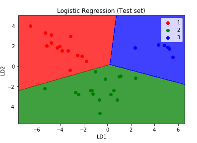
Linear Discriminant Analysis (LDA)

Basics:

From m independent variables of given dataset, LDA extracts p <= m new independent variables that separate most of the classes of the dependent variables.

Linear discriminant analysis (LDA) is a generalization of Fisher's linear discriminant, a method used in statistics, pattern recognition and machine learning to find a linear combination of features that characterizes or separates two or more classes of objects or events.

LDA is also closely related to PCA in that they both look for linear combinations of variables which best explain the data.

• LDA explicitly attempts to model the difference between the classes of data. 
• PCA on the other hand does not take into account any difference in class

Business Problem: 

(Same as in PCA) Given 13 independent variables (various type of alcohol) in wine, decide which customer segment will prefer a particular type of wine. Now as it's tough to determine customer segment on bases of so many independent variables, we'll apply PCA and deduce best two  independent variables to solve this problem.

Code: LDA

# Importing the libraries
import numpy as np
import matplotlib.pyplot as plt
import pandas as pd

# Importing the dataset
dataset = pd.read_csv('Wine.csv')
X = dataset.iloc[:, 0:13].values
y = dataset.iloc[:, 13].values

# Splitting the dataset into the Training set and Test set
from sklearn.model_selection import train_test_split
X_train, X_test, y_train, y_test = train_test_split(X, y, test_size = 0.2, random_state = 0)

# Feature Scaling
from sklearn.preprocessing import StandardScaler
sc = StandardScaler()
X_train = sc.fit_transform(X_train)
X_test = sc.transform(X_test)

# Applying LDA
from sklearn.discriminant_analysis import LinearDiscriminantAnalysis as LDA
lda = LDA(n_components = 2)
X_train = lda.fit_transform(X_train, y_train)  # This is additional here in comparison to LCA
X_test = lda.transform(X_test)

# Fitting Logistic Regression to the Training set
from sklearn.linear_model import LogisticRegression
classifier = LogisticRegression(random_state = 0)
classifier.fit(X_train, y_train)

# Predicting the Test set results
y_pred = classifier.predict(X_test)

# Making the Confusion Matrix
# Used to evauate performance of model to see corret/incorrection predictions made by Logistic regression
from sklearn.metrics import confusion_matrix
cm = confusion_matrix(y_test, y_pred)

# Visualising the Training set results
from matplotlib.colors import ListedColormap
X_set, y_set = X_train, y_train
X1, X2 = np.meshgrid(np.arange(start = X_set[:, 0].min() - 1, stop = X_set[:, 0].max() + 1, step = 0.01),
                     np.arange(start = X_set[:, 1].min() - 1, stop = X_set[:, 1].max() + 1, step = 0.01))
plt.contourf(X1, X2, classifier.predict(np.array([X1.ravel(), X2.ravel()]).T).reshape(X1.shape),
             alpha = 0.75, cmap = ListedColormap(('red', 'green', 'blue')))
plt.xlim(X1.min(), X1.max())
plt.ylim(X2.min(), X2.max())
for i, j in enumerate(np.unique(y_set)):
    plt.scatter(X_set[y_set == j, 0], X_set[y_set == j, 1],
                c = ListedColormap(('red', 'green', 'blue'))(i), label = j)
plt.title('Logistic Regression (Training set)')
plt.xlabel('LD1')
plt.ylabel('LD2')
plt.legend()
plt.show()

# Visualising the Test set results
from matplotlib.colors import ListedColormap
X_set, y_set = X_test, y_test
X1, X2 = np.meshgrid(np.arange(start = X_set[:, 0].min() - 1, stop = X_set[:, 0].max() + 1, step = 0.01),
                     np.arange(start = X_set[:, 1].min() - 1, stop = X_set[:, 1].max() + 1, step = 0.01))
plt.contourf(X1, X2, classifier.predict(np.array([X1.ravel(), X2.ravel()]).T).reshape(X1.shape),
             alpha = 0.75, cmap = ListedColormap(('red', 'green', 'blue')))
plt.xlim(X1.min(), X1.max())
plt.ylim(X2.min(), X2.max())
for i, j in enumerate(np.unique(y_set)):
    plt.scatter(X_set[y_set == j, 0], X_set[y_set == j, 1],
                c = ListedColormap(('red', 'green', 'blue'))(i), label = j)
plt.title('Logistic Regression (Test set)')
plt.xlabel('LD1')
plt.ylabel('LD2')
plt.legend()
plt.show()

Hope this helps!!

Arun Manglick

Principal Component Analysis (PCA)

Basics:

From m independent variables of given dataset, PCA extracts p <= m new independent variables that explain most of the variance of the dataset, regardless of the dependent variables.

Principal component analysis (PCA) is a statistical procedure that uses an orthogonal transformation to convert a set of observations of possibly correlated variables into a set of values of linearly uncorrelated variables called Principal Components (or sometimes, principal modes of variation).

The number of principal components is less than or equal to the smaller of the number of original variables or the number of observations.

This transformation is defined in such a way that the first principal component has the largest possible variance (that is, accounts for as much of the variability in the data as possible), and each succeeding component in turn has the highest variance possible under the constraint that it is orthogonal to the preceding components. The resulting vectors are an uncorrelated orthogonal basis set. PCA is sensitive to the relative scaling of the original variables.

Business Problem: 

Given 13 independent variables (various type of alcohol) in wine, decide which customer segment will prefer a particular type of wine. Now as it's tough to determine customer segment on bases of so many independent variables, we'll apply PCA and deduce best two  independent variables to solve this problem.

Code: PCA

# Importing the libraries
import numpy as np
import matplotlib.pyplot as plt
import pandas as pd

# Importing the dataset
dataset = pd.read_csv('Wine.csv')
X = dataset.iloc[:, 0:13].values
y = dataset.iloc[:, 13].values

# Splitting the dataset into the Training set and Test set
from sklearn.model_selection import train_test_split
X_train, X_test, y_train, y_test = train_test_split(X, y, test_size = 0.2, random_state = 0)

# Feature Scaling
from sklearn.preprocessing import StandardScaler
sc = StandardScaler()
X_train = sc.fit_transform(X_train)
X_test = sc.transform(X_test)

# Applying PCA
from sklearn.decomposition import PCA
# It extracts two principal component variables which has largest variance.
pca = PCA(n_components = 2)  
X_train = pca.fit_transform(X_train)
X_test = pca.transform(X_test)
explained_variance = pca.explained_variance_ratio_

# Fitting Logistic Regression to the Training set
from sklearn.linear_model import LogisticRegression
classifier = LogisticRegression(random_state = 0)
classifier.fit(X_train, y_train)

# Predicting the Test set results
y_pred = classifier.predict(X_test)

# Making the Confusion Matrix
# Used to evauate performance of model to see corret/incorrection predictions made by Logistic regression
from sklearn.metrics import confusion_matrix
cm = confusion_matrix(y_test, y_pred)

# Visualising the Training set results
from matplotlib.colors import ListedColormap
X_set, y_set = X_train, y_train
X1, X2 = np.meshgrid(np.arange(start = X_set[:, 0].min() - 1, stop = X_set[:, 0].max() + 1, step = 0.01),
                     np.arange(start = X_set[:, 1].min() - 1, stop = X_set[:, 1].max() + 1, step = 0.01))
plt.contourf(X1, X2, classifier.predict(np.array([X1.ravel(), X2.ravel()]).T).reshape(X1.shape),
             alpha = 0.75, cmap = ListedColormap(('red', 'green', 'blue')))
plt.xlim(X1.min(), X1.max())
plt.ylim(X2.min(), X2.max())
for i, j in enumerate(np.unique(y_set)):
    plt.scatter(X_set[y_set == j, 0], X_set[y_set == j, 1],
                c = ListedColormap(('red', 'green', 'blue'))(i), label = j)
plt.title('Logistic Regression (Training set)')
plt.xlabel('PC1')
plt.ylabel('PC2')
plt.legend()
plt.show()

# Visualising the Test set results
from matplotlib.colors import ListedColormap
X_set, y_set = X_test, y_test
X1, X2 = np.meshgrid(np.arange(start = X_set[:, 0].min() - 1, stop = X_set[:, 0].max() + 1, step = 0.01),
                     np.arange(start = X_set[:, 1].min() - 1, stop = X_set[:, 1].max() + 1, step = 0.01))
plt.contourf(X1, X2, classifier.predict(np.array([X1.ravel(), X2.ravel()]).T).reshape(X1.shape),
             alpha = 0.75, cmap = ListedColormap(('red', 'green', 'blue')))
plt.xlim(X1.min(), X1.max())
plt.ylim(X2.min(), X2.max())
for i, j in enumerate(np.unique(y_set)):
    plt.scatter(X_set[y_set == j, 0], X_set[y_set == j, 1],
                c = ListedColormap(('red', 'green', 'blue'))(i), label = j)
plt.title('Logistic Regression (Test set)')
plt.xlabel('PC1')
plt.ylabel('PC2')
plt.legend()
plt.show()

Hope this helps!!

Arun Manglick

Part 9: Dimensionality Reduction

Basics:

In Classification, we worked with datasets composed of only two independent variables.
Two dimensions visualize better how Machine Learning models worked (by plotting the prediction regions and the prediction boundary for each model).

In case where there are more than two independent variables, we can often end up with two independent variables by applying an appropriate Dimensionality Reduction technique.

There are two types of Dimensionality Reduction techniques:

1. Feature Selection - Covered in Part 2 - Regression.
• Backward Elimination, 
• Forward Selection, 
• Bidirectional Elimination, 
• Score Comparison
2. Feature Extraction 
• Principal Component Analysis (PCA)  - Works on Linear Separable Model
• Linear Discriminant Analysis (LDA)  - Works on Linear Separable Model
• Kernel PCA  - Works on Non-Linear Separable  Model
• Quadratic Discriminant Analysis (QDA)

We'll cover Feature Extraction techniques here.

Hope this helps!!!

Arun Manglick