Basics:
Here we'll first learn below:


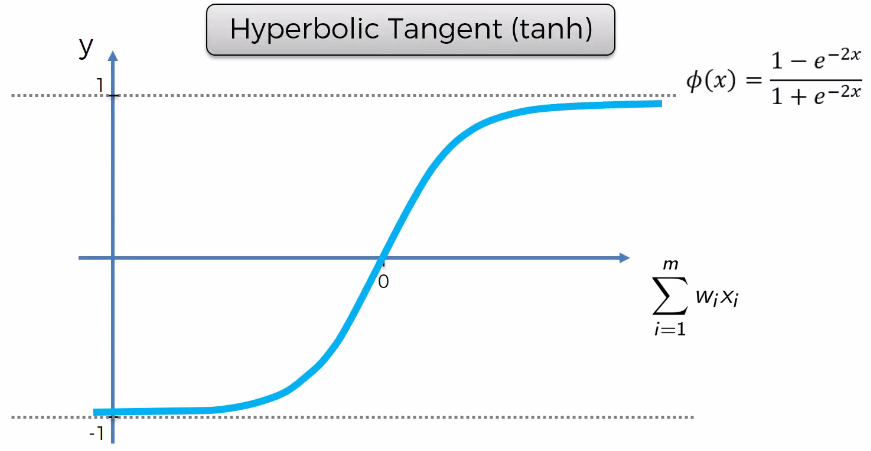
Four Types:
- Threshold Function (Passes 0 or 1, If X < 0, Then 0, If X >= 0 Then 1)
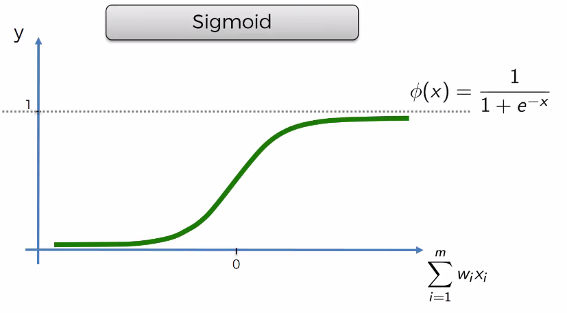
- Sigmoid Function (Used in Logistic Regression)
- Rectifier Function (Mostly Used) (Paper Link)
- Hyperbolic Tanget (tanh)

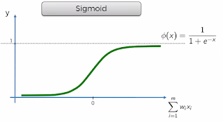

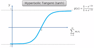
In most of the model, Rectifier is applied at 2nd step and Sigmoid is at 3rd step.

3). How Neuron Network Learns:
Steps:


4). Gradient Descent:
Gradient descent is a popular method in the field of machine learning and used to find the minimum error by minimizing a "cost" function.
Gradient descent is a first-order iterative optimization algorithm for finding the minimum of a function.
To find a local minimum of a function using gradient descent, one takes steps proportional to the negative of the gradient (or of the approximate gradient) of the function at the current point. If instead one takes steps proportional to the positive of the gradient, one approaches a local maximum of that function; the procedure is then known as gradient ascent.
In easy words to find minimum, move in the way whichever is downhill, take steps and find minimum faster.


5). Stochastic Gradient Descent:
Above is able to find a global minimum where cross function is convex. But what if it's not convex and look like below. In this case, as you see applying above method ends up with incorrect minimum point.

In such case SGD is used.
Stochastic gradient descent (often shortened in SGD), also known as incremental gradient descent, is a stochastic approximation of the gradient descent optimization method for minimizing an objective function that is written as a sum of differentiable functions. In other words, SGD tries to find minima or maxima by iteration.

6). Back Propogation:

Practical:
Here we'll understand below:
1). Business Problem:
You have bank customers (credit score, country, age, gender, tenure,balance, credit card, loan, exited etc). Given the problem you need to find out which customers are at high risk of leaving the bank.
In summary, it's a Classification Problem.
2). Installation/Understand Theano, TensorFlow, Keras
Theano: At a glance
Theano is an open source numerical computation Python library that allows you to Define, Optimize, and Evaluate mathematical expressions involving multi-dimensional arrays efficiently. Theano can run on CPU or GPU (more useful for neural networks calculations).
Features:
TensorFlow is an open source software library for numerical computation using data flow graphs. Nodes in the graph represent mathematical operations, while the graph edges represent the multidimensional data arrays (tensors) communicated between them.
The flexible architecture allows you to deploy computation to one or more CPUs or GPUs in a desktop, server, or mobile device with a single API.
TensorFlow computations are expressed as stateful dataflow graphs. The name TensorFlow derives from the operations which such neural networks perform on multidimensional data arrays (tensors).
TensorFlow was originally developed by researchers and engineers working on the Google Brain Team (Nov 2015) for the purposes of conducting machine learning and deep neural networks research.
Used for machine learning across a range of tasks, building and training neural networks to detect and decipher patterns and correlations, analogous to the learning and reasoning which humans use.
In just its first year, TensorFlow has helped researchers, engineers, artists, students, and many others make progress with everything from language translation to early detection of skin cancer and preventing blindness in diabetics.
Keras:
Keras was developed with a focus on enabling fast experimentation.
Keras library is used to build deep neural network model with very few lines of code.
Keras is a high-level neural networks API, written in Python and capable of running on top of TensorFlow, Theano, MXNet, Deeplearning4j or CNTK.
Google's (In 2017) TensorFlow team decided to support Keras in TensorFlow's core library. It was explained that Keras was conceived to be an interface rather than an end-to-end machine-learning framework. It presents a higher-level, more intuitive set of abstractions that make it easy to configure neural networks regardless of the backend scientific computing library.
Microsoft has been working to add a CNTK backend to Keras as well.
The library contains numerous implementations of commonly used neural network building blocks such as layers, objectives, activation functions, optimizers, and a host of tools to make working with image and text data easier.
Code: Artificial Neural Network
# Part 1: Data Pre-Processing
# Importing the libraries
import numpy as np
import matplotlib.pyplot as plt
import pandas as pd
# Importing the dataset
dataset = pd.read_csv('Churn_Modelling.csv')
X = dataset.iloc[:, 3:13].values
y = dataset.iloc[:, 13].values
# Encoding categorical data - 'Geography'& 'Gender'
from sklearn.preprocessing import LabelEncoder, OneHotEncoder
labelencoder_X_1 = LabelEncoder()
X[:, 1] = labelencoder_X_1.fit_transform(X[:, 1])
labelencoder_X_2 = LabelEncoder()
X[:, 2] = labelencoder_X_2.fit_transform(X[:, 2])
onehotencoder = OneHotEncoder(categorical_features = [1])
X = onehotencoder.fit_transform(X).toarray()
X = X[:, 1:] # To avoid dummy variable trap
# Splitting the dataset into the Training set and Test set
from sklearn.model_selection import train_test_split
X_train, X_test, y_train, y_test = train_test_split(X, y, test_size = 0.2, random_state = 0)
# Feature Scaling
from sklearn.preprocessing import StandardScaler
sc = StandardScaler()
X_train = sc.fit_transform(X_train)
X_test = sc.transform(X_test)
# Part2: Now let's make the ANN!
# Importing the Keras libraries and packages
import keras
from keras.models import Sequential
from keras.layers import Dense
# Initializing the ANN
classifier = Sequential()
# Adding the input layer and the first hidden layer
# Here Output_dim denotes number of hidden layers, which is taken as average of input & outout. I.e (11+1)/2 = 6
# Here we are choosing 'Rectifier' (relu) as an activation function for Hidden Layer
# Here we are choosing 'Sigmoid' as an activation function for Output Layer
classifier.add(Dense(output_dim = 6, init = 'uniform', activation = 'relu', input_dim = 11))
# Adding the second hidden layer
classifier.add(Dense(output_dim = 6, init = 'uniform', activation = 'relu'))
# Adding the output layer
classifier.add(Dense(output_dim = 1, init = 'uniform', activation = 'sigmoid'))
# Compiling the ANN
# Here optimizer is 'Stochastic Gradient Descent'. One of the SGD Algoritm is 'adam'
classifier.compile(optimizer = 'adam', loss = 'binary_crossentropy', metrics = ['accuracy'])
classifier.compile()
# Fitting the ANN to the Training set
classifier.fit(X_train, y_train, batch_size = 10, nb_epoch = 100)
# Part 3 - Making the predictions and evaluating the model
# Predicting the Test set results
y_pred = classifier.predict(X_test)
y_pred = (y_pred > 0.5) # Predictions Less Than 0.5 will be treated as 'False', else 'True'
# Making the Confusion Matrix
from sklearn.metrics import confusion_matrix
cm = confusion_matrix(y_test, y_pred)
Hope this helps!!
Here we'll first learn below:
- Neuron
- Activation Function
- How Neural N/w Learn
- Gradient Descent
- Stochastic Gradient Descent
- Back Propagation
1). Neuron:


2). Activation Function:
Four Types:
- Threshold Function (Passes 0 or 1, If X < 0, Then 0, If X >= 0 Then 1)
- Sigmoid Function (Used in Logistic Regression)
- Rectifier Function (Mostly Used) (Paper Link)
- Hyperbolic Tanget (tanh)


In most of the model, Rectifier is applied at 2nd step and Sigmoid is at 3rd step.

3). How Neuron Network Learns:
Steps:
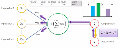
- Apply Weight to Input Values and Calculate Output Values (y Hat)
- Determine Cost I.e. variation between actual value (y) and predicted value (y hat)
- Intent is to minimize cost as much as possible. Thus adjust weight and re-apply and check new cost value
- Repeat steps until you find zero or minimum cost value


The above is applied to one student. If there are multiple student same is applied to all rows in one go and repeated again for all rows in one go, until you find cumulative minimum cost.

4). Gradient Descent:
Gradient descent is a popular method in the field of machine learning and used to find the minimum error by minimizing a "cost" function.
Gradient descent is a first-order iterative optimization algorithm for finding the minimum of a function.
To find a local minimum of a function using gradient descent, one takes steps proportional to the negative of the gradient (or of the approximate gradient) of the function at the current point. If instead one takes steps proportional to the positive of the gradient, one approaches a local maximum of that function; the procedure is then known as gradient ascent.
In easy words to find minimum, move in the way whichever is downhill, take steps and find minimum faster.


5). Stochastic Gradient Descent:
Above is able to find a global minimum where cross function is convex. But what if it's not convex and look like below. In this case, as you see applying above method ends up with incorrect minimum point.

In such case SGD is used.
Stochastic gradient descent (often shortened in SGD), also known as incremental gradient descent, is a stochastic approximation of the gradient descent optimization method for minimizing an objective function that is written as a sum of differentiable functions. In other words, SGD tries to find minima or maxima by iteration.

6). Back Propogation:

Practical:
Here we'll understand below:
- Business Problem
- Installing/Understand
- Theano,
- Tensorflow and
- Keras
- Code Implementation
1). Business Problem:
You have bank customers (credit score, country, age, gender, tenure,balance, credit card, loan, exited etc). Given the problem you need to find out which customers are at high risk of leaving the bank.
In summary, it's a Classification Problem.
2). Installation/Understand Theano, TensorFlow, Keras
Theano: At a glance
Theano is an open source numerical computation Python library that allows you to Define, Optimize, and Evaluate mathematical expressions involving multi-dimensional arrays efficiently. Theano can run on CPU or GPU (more useful for neural networks calculations).
Features:
- Tight integration with NumPy - e.g. Theano can use g++ or nvcc to compile parts your expression graph into CPU or GPU instructions, which run much faster than pure Python.
- Transparent use of a GPU – Perform data-intensive computations much faster than on a CPU.
- Efficient symbolic differentiation – Theano can automatically build symbolic graphs for computing gradients.
- Speed and stability optimizations – Get the right answer for log(1+x) even when x is really tiny.
- Dynamic C code generation – Evaluate expressions faster.
- Extensive unit-testing and self-verification – Detect and diagnose many types of errors.
TensorFlow is an open source software library for numerical computation using data flow graphs. Nodes in the graph represent mathematical operations, while the graph edges represent the multidimensional data arrays (tensors) communicated between them.
The flexible architecture allows you to deploy computation to one or more CPUs or GPUs in a desktop, server, or mobile device with a single API.
TensorFlow computations are expressed as stateful dataflow graphs. The name TensorFlow derives from the operations which such neural networks perform on multidimensional data arrays (tensors).
TensorFlow was originally developed by researchers and engineers working on the Google Brain Team (Nov 2015) for the purposes of conducting machine learning and deep neural networks research.
Used for machine learning across a range of tasks, building and training neural networks to detect and decipher patterns and correlations, analogous to the learning and reasoning which humans use.
In just its first year, TensorFlow has helped researchers, engineers, artists, students, and many others make progress with everything from language translation to early detection of skin cancer and preventing blindness in diabetics.
Keras:
Keras was developed with a focus on enabling fast experimentation.
Keras library is used to build deep neural network model with very few lines of code.
Keras is a high-level neural networks API, written in Python and capable of running on top of TensorFlow, Theano, MXNet, Deeplearning4j or CNTK.
Google's (In 2017) TensorFlow team decided to support Keras in TensorFlow's core library. It was explained that Keras was conceived to be an interface rather than an end-to-end machine-learning framework. It presents a higher-level, more intuitive set of abstractions that make it easy to configure neural networks regardless of the backend scientific computing library.
Microsoft has been working to add a CNTK backend to Keras as well.
The library contains numerous implementations of commonly used neural network building blocks such as layers, objectives, activation functions, optimizers, and a host of tools to make working with image and text data easier.
Code: Artificial Neural Network
# Part 1: Data Pre-Processing
# Importing the libraries
import numpy as np
import matplotlib.pyplot as plt
import pandas as pd
# Importing the dataset
dataset = pd.read_csv('Churn_Modelling.csv')
X = dataset.iloc[:, 3:13].values
y = dataset.iloc[:, 13].values
# Encoding categorical data - 'Geography'& 'Gender'
from sklearn.preprocessing import LabelEncoder, OneHotEncoder
labelencoder_X_1 = LabelEncoder()
X[:, 1] = labelencoder_X_1.fit_transform(X[:, 1])
labelencoder_X_2 = LabelEncoder()
X[:, 2] = labelencoder_X_2.fit_transform(X[:, 2])
onehotencoder = OneHotEncoder(categorical_features = [1])
X = onehotencoder.fit_transform(X).toarray()
X = X[:, 1:] # To avoid dummy variable trap
# Splitting the dataset into the Training set and Test set
from sklearn.model_selection import train_test_split
X_train, X_test, y_train, y_test = train_test_split(X, y, test_size = 0.2, random_state = 0)
# Feature Scaling
from sklearn.preprocessing import StandardScaler
sc = StandardScaler()
X_train = sc.fit_transform(X_train)
X_test = sc.transform(X_test)
# Part2: Now let's make the ANN!
# Importing the Keras libraries and packages
import keras
from keras.models import Sequential
from keras.layers import Dense
# Initializing the ANN
classifier = Sequential()
# Adding the input layer and the first hidden layer
# Here Output_dim denotes number of hidden layers, which is taken as average of input & outout. I.e (11+1)/2 = 6
# Here we are choosing 'Rectifier' (relu) as an activation function for Hidden Layer
# Here we are choosing 'Sigmoid' as an activation function for Output Layer
classifier.add(Dense(output_dim = 6, init = 'uniform', activation = 'relu', input_dim = 11))
# Adding the second hidden layer
classifier.add(Dense(output_dim = 6, init = 'uniform', activation = 'relu'))
# Adding the output layer
classifier.add(Dense(output_dim = 1, init = 'uniform', activation = 'sigmoid'))
# Compiling the ANN
# Here optimizer is 'Stochastic Gradient Descent'. One of the SGD Algoritm is 'adam'
classifier.compile(optimizer = 'adam', loss = 'binary_crossentropy', metrics = ['accuracy'])
classifier.compile()
# Fitting the ANN to the Training set
classifier.fit(X_train, y_train, batch_size = 10, nb_epoch = 100)
# Part 3 - Making the predictions and evaluating the model
# Predicting the Test set results
y_pred = classifier.predict(X_test)
y_pred = (y_pred > 0.5) # Predictions Less Than 0.5 will be treated as 'False', else 'True'
# Making the Confusion Matrix
from sklearn.metrics import confusion_matrix
cm = confusion_matrix(y_test, y_pred)
Hope this helps!!
Arun Manglick
Thanks for sharing nice post..
ReplyDeleteMachine Learning Online Training
Machine Learning Online Course