Basics:
In data mining and statistics, Hierarchical Clustering (also called Hierarchical Cluster Analysis or HCA) is a method of cluster analysis which seeks to build a Hierarchy of Clusters. Strategies for hierarchical clustering generally fall into two types.
Here are various options to calculate 'Distance Between Two Clusters'.

Let's apply above steps.


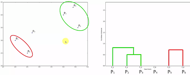
Intent of going this obvious easy steps is it maintains the steps how we proceed in memory and then the memory is stored in a 'Dendograms'. Here is how Dendograms are generated.
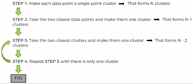
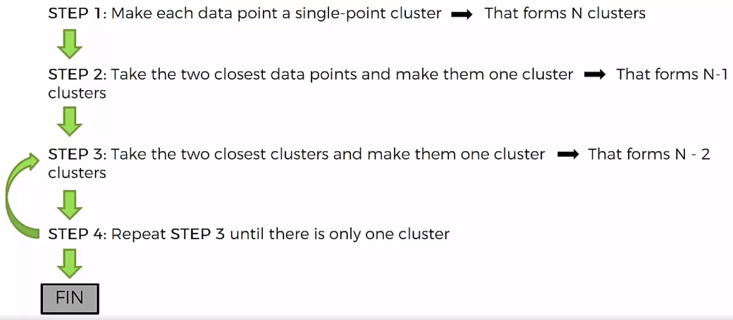
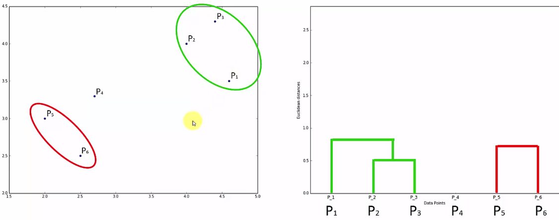
- Step 1: Combine closer data points and make one cluster (Left) and for this cluster draw as in right (here height will be decided by the distance) between two points.
- Step 2: Repeat this step until you come up with single cluster.
- Step 3:Check for longest vertical lines not crossing any horizontal lines. That will determine the number of clusters. Here in our case 2 Clusters will be the optimum one.


One more example:

Code: Hierarchical Clustering
# For the given problem Age, Salary and Spending score, below code will try to deduce how many customer segments can be created so that business can focus on those segments and create corrective business plans.
# Importing the libraries
import numpy as np
import matplotlib.pyplot as plt
import pandas as pd
# Importing the dataset
dataset = pd.read_csv('Mall_Customers.csv')
X = dataset.iloc[:, [3, 4]].values
# y = dataset.iloc[:, 3].values
# Using the dendrogram to find the optimal number of clusters
import scipy.cluster.hierarchy as sch
dendrogram = sch.dendrogram(sch.linkage(X, method = 'ward'))
plt.title('Dendrogram')
plt.xlabel('Customers')
plt.ylabel('Euclidean distances')
plt.show()
 # Fitting Hierarchical Clustering to the dataset
from sklearn.cluster import AgglomerativeClustering
hc = AgglomerativeClustering(n_clusters = 5, affinity = 'euclidean', linkage = 'ward')
y_hc = hc.fit_predict(X)
# Visualising the clusters
plt.scatter(X[y_hc == 0, 0], X[y_hc == 0, 1], s = 100, c = 'red', label = 'Cluster 1')
plt.scatter(X[y_hc == 1, 0], X[y_hc == 1, 1], s = 100, c = 'blue', label = 'Cluster 2')
plt.scatter(X[y_hc == 2, 0], X[y_hc == 2, 1], s = 100, c = 'green', label = 'Cluster 3')
plt.scatter(X[y_hc == 3, 0], X[y_hc == 3, 1], s = 100, c = 'cyan', label = 'Cluster 4')
plt.scatter(X[y_hc == 4, 0], X[y_hc == 4, 1], s = 100, c = 'magenta', label = 'Cluster 5')
plt.title('Clusters of customers')
plt.xlabel('Annual Income (k$)')
plt.ylabel('Spending Score (1-100)')
plt.legend()
plt.show()

Cluster 1 - More Income & Less Spending - Careful Clients
Cluster 2 - Average Income & Average Spending - Standard Clients
Cluster 3 - High Income & High Spending - Potential Clients
Cluster 4 - Less Income & High Spending - Careless Clients
Cluster 5 - Less Income & Less Spending - Sensible Clients
Hope this helps!!
Arun Manglick
In data mining and statistics, Hierarchical Clustering (also called Hierarchical Cluster Analysis or HCA) is a method of cluster analysis which seeks to build a Hierarchy of Clusters. Strategies for hierarchical clustering generally fall into two types.
- Agglomerative: This is a "bottom up" approach: each observation starts in its own cluster, and pairs of clusters are merged as one moves up the hierarchy.
- Divisive: This is a "top down" approach: all observations start in one cluster, and splits are performed recursively as one moves down the hierarchy.
Here are various options to calculate 'Distance Between Two Clusters'.

Let's apply above steps.


Intent of going this obvious easy steps is it maintains the steps how we proceed in memory and then the memory is stored in a 'Dendograms'. Here is how Dendograms are generated.
- Step 1: Combine closer data points and make one cluster (Left) and for this cluster draw as in right (here height will be decided by the distance) between two points.
- Step 2: Repeat this step until you come up with single cluster.
- Step 3:Check for longest vertical lines not crossing any horizontal lines. That will determine the number of clusters. Here in our case 2 Clusters will be the optimum one.


One more example:

Code: Hierarchical Clustering
# For the given problem Age, Salary and Spending score, below code will try to deduce how many customer segments can be created so that business can focus on those segments and create corrective business plans.
# Importing the libraries
import numpy as np
import matplotlib.pyplot as plt
import pandas as pd
# Importing the dataset
dataset = pd.read_csv('Mall_Customers.csv')
X = dataset.iloc[:, [3, 4]].values
# y = dataset.iloc[:, 3].values
# Using the dendrogram to find the optimal number of clusters
import scipy.cluster.hierarchy as sch
dendrogram = sch.dendrogram(sch.linkage(X, method = 'ward'))
plt.title('Dendrogram')
plt.xlabel('Customers')
plt.ylabel('Euclidean distances')
plt.show()

from sklearn.cluster import AgglomerativeClustering
hc = AgglomerativeClustering(n_clusters = 5, affinity = 'euclidean', linkage = 'ward')
y_hc = hc.fit_predict(X)
# Visualising the clusters
plt.scatter(X[y_hc == 0, 0], X[y_hc == 0, 1], s = 100, c = 'red', label = 'Cluster 1')
plt.scatter(X[y_hc == 1, 0], X[y_hc == 1, 1], s = 100, c = 'blue', label = 'Cluster 2')
plt.scatter(X[y_hc == 2, 0], X[y_hc == 2, 1], s = 100, c = 'green', label = 'Cluster 3')
plt.scatter(X[y_hc == 3, 0], X[y_hc == 3, 1], s = 100, c = 'cyan', label = 'Cluster 4')
plt.scatter(X[y_hc == 4, 0], X[y_hc == 4, 1], s = 100, c = 'magenta', label = 'Cluster 5')
plt.title('Clusters of customers')
plt.xlabel('Annual Income (k$)')
plt.ylabel('Spending Score (1-100)')
plt.legend()
plt.show()

Cluster 1 - More Income & Less Spending - Careful Clients
Cluster 2 - Average Income & Average Spending - Standard Clients
Cluster 3 - High Income & High Spending - Potential Clients
Cluster 4 - Less Income & High Spending - Careless Clients
Cluster 5 - Less Income & Less Spending - Sensible Clients
Hope this helps!!
Arun Manglick
No comments:
Post a Comment