Random Forest : Regression

Basics:

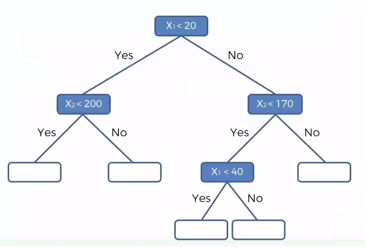
Random forests or random decision forests are an Ensemble learning method (Applying same algorithm multiple times) for classification, regression and other tasks, that operate by constructing a multitude of decision trees at training time and outputting the class that is the mode of the classes (classification) or mean prediction (regression) of the individual trees.

Random forests are a way of averaging multiple deep decision trees, trained on different parts of the same training set, with the goal of reducing the variance.

Code: Random Forest Regression

# Importing the libraries
import numpy as np
import matplotlib.pyplot as plt
import pandas as pd

# Importing the dataset
dataset = pd.read_csv('Position_Salaries.csv')
X = dataset.iloc[:, 1:2].values
y = dataset.iloc[:, 2].values

# Splitting the dataset into the Training set and Test set (Not Required)
"""from sklearn.cross_validation import train_test_split
X_train, X_test, y_train, y_test = train_test_split(X, y, test_size = 0.2, random_state = 0)"""

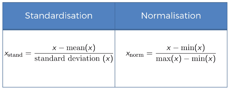
# Feature Scaling  (Not Required)
"""from sklearn.preprocessing import StandardScaler
sc_X = StandardScaler()
X_train = sc_X.fit_transform(X_train)
X_test = sc_X.transform(X_test)
sc_y = StandardScaler()
y_train = sc_y.fit_transform(y_train)"""

# Fitting Random Forest Regression to the dataset
from sklearn.ensemble import RandomForestRegressor
regressor = RandomForestRegressor(n_estimators = 10, random_state = 0)
regressor.fit(X, y)

# Converting X, Y in a range of .01 for higher resolution and  smoother curve
X_grid = np.arange(min(X), max(X), 0.01)
X_grid = X_grid.reshape((len(X_grid), 1))

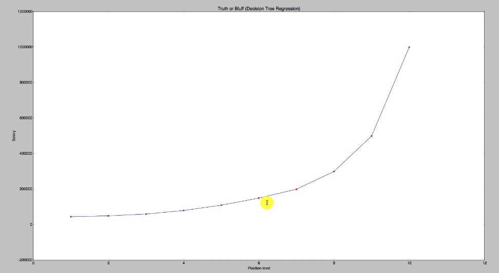
# Visualising the Random Forest Regression results (higher resolution)
plt.scatter(X, y, color = 'red')
plt.plot(X_grid, regressor.predict(X_grid), color = 'blue')
plt.title('Truth or Bluff (Random Forest Regression)')
plt.xlabel('Position level')
plt.ylabel('Salary')
plt.show()

Hope this helps!!

Arun Manglick

Decision Tree : Regression

Basics:

The term Classification And Regression Tree (CART) analysis is an umbrella term used to refer two types of Decision Trees, used in data mining:

• Classification tree analysis is when the predicted outcome is the class to which the data belongs.(Male/Female, Apple/Orange, Yes/No etc)
• Regression tree analysis is when the predicted outcome can be considered a real number (e.g. the price of a house, or a patient's length of stay in a hospital).

Here we'll talk about Regression Trees.
Regression Trees are more complex than Classification.

Decision tree learning is a method commonly used in data mining.The goal is to create a model that predicts the value of a target variable based on several input variables. This is achieved by Splitting the source dataset.

In mathematical form:
(x,Y)=(x1,x2,x3,...,xk,Y)

The dependent variable, Y, is the target variable that we are trying to understand, classify or generalize. The vector x is composed of the input variables, x1, x2, x3 etc., that are used for that task.

A tree can be "learned" by splitting the source set into subsets based on an attribute value test. This process is repeated on each derived subset in a recursive manner called recursive partitioning. The recursion is completed when the subset at a node has all the same value of the target variable, or when splitting no longer adds value to the predictions. This process of top-down induction of decision trees (TDIDT) is an example of a greedy algorithm, and it is by far the most common strategy for learning decision trees from data.

Consider the below source dataset having non-linear values or multiple (for e.g) two input variables (x1,x2).

To deduce the value on dependent variable (y), decision tree algorithm splits the data as mentioned above (I.e. Split till a particular area has same value of the target variable, or when splitting no longer adds value to the predictions).

Below will be it's Decision tree:

Now to predict value of Y, for any new point (x1,x2) lying in a particular split, you take average of all the points in a particular split and that average will be the value of Y, for that new point (x1,x2). 

Example: Say X1:30 & X2: 50, Y will be 64.1, as the new points (x1,X2) lies in that split.

Code: Decision Tree Regression

# Importing the libraries
import numpy as np
import matplotlib.pyplot as plt
import pandas as pd

# Importing the dataset
dataset = pd.read_csv('Position_Salaries.csv')
X = dataset.iloc[:, 1:2].values
y = dataset.iloc[:, 2].values

# Splitting the dataset into the Training set and Test set is skipped due the dataset size is just 10 rows
"""from sklearn.cross_validation import train_test_split
X_train, X_test, y_train, y_test = train_test_split(X, y, test_size = 0.2, random_state = 0)"""

# Feature Scaling (Not Required here)
"""from sklearn.preprocessing import StandardScaler
sc_X = StandardScaler()
X_train = sc_X.fit_transform(X_train)
X_test = sc_X.transform(X_test)
sc_y = StandardScaler()
y_train = sc_y.fit_transform(y_train)"""

# Fitting Decision Tree Regression to the dataset (Fig 1)
from sklearn.tree import DecisionTreeRegressor
regressor = DecisionTreeRegressor(random_state = 0)
regressor.fit(X, y)

# Visualising the Decision Tree Regression results (higher resolution)
X_grid = np.arange(min(X), max(X), 0.01)
X_grid = X_grid.reshape((len(X_grid), 1))

# Re-Visualising the Decision Tree Regression results 
plt.scatter(X, y, color = 'red')
plt.plot(X_grid, regressor.predict(X_grid), color = 'blue')
plt.title('Truth or Bluff (Decision Tree Regression)')
plt.xlabel('Position level')
plt.ylabel('Salary')
plt.show()

Hope this helps!!!

Arun Manglick

Support Vector Regression (SVR)

Code: SVR

# Importing the libraries
import numpy as np
import matplotlib.pyplot as plt
import pandas as pd

# Importing the dataset
dataset = pd.read_csv('Position_Salaries.csv')
X = dataset.iloc[:, 1:2].values  # Only one column taken
y = dataset.iloc[:, 2].values

# Splitting the dataset into the Training set and Test set is skipped due the dataset size is just 10 rows
"""from sklearn.cross_validation import train_test_split
X_train, X_test, y_train, y_test = train_test_split(X, y, test_size = 0.2, random_state = 0)"""

# Feature Scaling (Unlike Polynomial, scaling is required here as SVR library do not have in-build scaling. Without this plot will look like as in Fig 1, flat line)
from sklearn.preprocessing import StandardScaler
sc_X = StandardScaler()
sc_y = StandardScaler()
X = sc_X.fit_transform(X)
y = sc_y.fit_transform(y)

# Fitting SVR to the dataset
# kernel : Specifies the kernel type to be used in the algorithm. 
# It must be one of ‘linear’, ‘poly’, ‘rbf’, ‘sigmoid’, ‘precomputed’ or a callable.
from sklearn.svm import SVR
regressor = SVR(kernel = 'rbf') # 'rbf' is non-linear
regressor.fit(X, y)

# Visualising the SVR results
plt.scatter(X, y, color = 'red')
plt.plot(X, regressor.predict(X), color = 'blue')
plt.title('Truth or Bluff (SVR)')
plt.xlabel('Position level')
plt.ylabel('Salary')
plt.show()

# Visualising the SVR results (for higher resolution and smoother curve)
X_grid = np.arange(min(X), max(X), 0.01) # choice of 0.01 instead of 0.1 step because the data is feature scaled
X_grid = X_grid.reshape((len(X_grid), 1))

# Re-Visualising the SVR results
plt.scatter(X, y, color = 'red')
plt.plot(X_grid, regressor.predict(X_grid), color = 'blue')
plt.title('Truth or Bluff (SVR)')
plt.xlabel('Position level')
plt.ylabel('Salary')
plt.show()

Fig 1.

Hope this helps!!

Regards,
Arun Manglick

Polynomial Linear Regression

Basics:

Why Polynomial Linear Regression required? I.e. Why can't problem be resolved thru just Simple/Multiple Linear?
Ans: For the data points like below, Simple/Multiple Linear Regression works fine (Fig 1). However if the data points are slightly parabolic, Simple/Multiple Linear Regression doesn't works well. (Fig 2). This is where  Polynomial Linear Regression fits well (Fig 3).

Fig 1.

Fig 2 (Not Fitting)

Fig 3.

Code: Polynomial Regression

# Importing the libraries
import numpy as np
import matplotlib.pyplot as plt
import pandas as pd

# Importing the dataset
dataset = pd.read_csv('Position_Salaries.csv')
X = dataset.iloc[:, 1:2].values   # Only one column taken
y = dataset.iloc[:, 2].values

# Splitting the dataset into the Training set and Test set is skipped due the dataset size is just 10 rows
"""from sklearn.cross_validation import train_test_split
X_train, X_test, y_train, y_test = train_test_split(X, y, test_size = 0.2, random_state = 0)"""

# Feature Scaling (Not required as data is already requires levels in designation)
"""from sklearn.preprocessing import StandardScaler
sc_X = StandardScaler()
X_train = sc_X.fit_transform(X_train)
X_test = sc_X.transform(X_test)"""

# Fitting Linear Regression to the dataset
from sklearn.linear_model import LinearRegression
lin_reg = LinearRegression()
lin_reg.fit(X, y)

# Fitting Polynomial Regression to the dataset
from sklearn.preprocessing import PolynomialFeatures
poly_reg = PolynomialFeatures(degree = 4)
X_poly = poly_reg.fit_transform(X)
poly_reg.fit(X_poly, y)

# Fitting Linear Regression to the Polynomial Result set
lin_reg_2 = LinearRegression()
lin_reg_2.fit(X_poly, y)

# Visualising the Linear Regression results
plt.scatter(X, y, color = 'red')
plt.plot(X, lin_reg.predict(X), color = 'blue')
plt.title('Truth or Bluff (Linear Regression)')
plt.xlabel('Position level')
plt.ylabel('Salary')
plt.show()



# Visualising the Polynomial Regression results
plt.scatter(X, y, color = 'red')
plt.plot(X, lin_reg_2.predict(poly_reg.fit_transform(X)), color = 'blue')
plt.title('Truth or Bluff (Polynomial Regression)')
plt.xlabel('Position level')
plt.ylabel('Salary')
plt.show()

# Visualising the Polynomial Regression results (for higher resolution and smoother curve)
# This is done for more smooth fitting the graph
X_grid = np.arange(min(X), max(X), 0.1)
X_grid = X_grid.reshape((len(X_grid), 1))

# Re-Visualising the Polynomial Regression results (on smoothened result set)
plt.scatter(X, y, color = 'red')
plt.plot(X_grid, lin_reg_2.predict(poly_reg.fit_transform(X_grid)), color = 'blue')
plt.title('Truth or Bluff (Polynomial Regression)')
plt.xlabel('Position level')
plt.ylabel('Salary')
plt.show()

Hope this helps!!!

Arun Manglick

Multiple Linear Regression

Basics:

Here is how Multiple Linear Regression (MLR) is defined in mathematics:
Here multiple independent variables are considered to drive one dependent variable. e.g. Student Grade(y) will be dependent on multiple variables, like Study Time (x1), Sleep Time (x2), School Time (x3) etc.

Dummy Variable Trap:

If there are multiple dummy variables, then in MLR equations, always omit one variable. I.e. if there are 100 dummy variables, then take 99 only.

Building Regression Model Approaches:

There are five methods of building regression model:

1. All-In (Take All Independent Variables(x1,x2,....xn))
2. Backward Elimination (Fastest of All)
3. Forward Selection
4. Bidirectional Elimination
5. Score Comparison

Code: Multiple Linear Regression

# Importing the libraries
import numpy as np
import matplotlib.pyplot as plt
import pandas as pd

# Importing the dataset
dataset = pd.read_csv('50_Startups.csv')
X = dataset.iloc[:, :-1].values
y = dataset.iloc[:, 4].values

# Encoding categorical data
from sklearn.preprocessing import LabelEncoder, OneHotEncoder
labelencoder = LabelEncoder()
X[:, 3] = labelencoder.fit_transform(X[:, 3])
onehotencoder = OneHotEncoder(categorical_features = [3])
X = onehotencoder.fit_transform(X).toarray()

# Avoiding the Dummy Variable Trap
X = X[:, 1:]

# Splitting the dataset into the Training set and Test set
from sklearn.cross_validation import train_test_split
X_train, X_test, y_train, y_test = train_test_split(X, y, test_size = 0.2, random_state = 0)

# Fitting Multiple Linear Regression to the Training set
from sklearn.linear_model import LinearRegression
regressor = LinearRegression()
regressor.fit(X_train, y_train)

# Predicting the Test set results
y_pred = regressor.predict(X_test)

# Building the optimal model using Backward Elimination
import statsmodels.formula.api as sm
# This add one column in start of all ones, to make X0 for b0 constant
X = np.append(arr = np.ones((50, 1)).astype(int), values = X, axis = 1)

X_opt = X[:, [0, 1, 2, 3, 4, 5]]
regressor_OLS = sm.OLS(endog = y, exog = X_opt).fit()
regressor_OLS.summary()

X_opt = X[:, [0, 1, 3, 4, 5]]
regressor_OLS = sm.OLS(endog = y, exog = X_opt).fit()
regressor_OLS.summary()

X_opt = X[:, [0, 3, 4, 5]]
regressor_OLS = sm.OLS(endog = y, exog = X_opt).fit()
regressor_OLS.summary()

X_opt = X[:, [0, 3, 5]]
regressor_OLS = sm.OLS(endog = y, exog = X_opt).fit()
regressor_OLS.summary()

X_opt = X[:, [0, 3]]
regressor_OLS = sm.OLS(endog = y, exog = X_opt).fit()
regressor_OLS.summary()


Hope this helps!!!

Arun Manglick

Simple Linear Regression

Basics:

Here is how Linear Regression (LR) is defined in mathematics:
Coefficient is also defined as 'Slope'. More the slope, more the hike in salary.

Ordinary Least Square (OLS):

LR applies OLS method to find the trend line.
Here Red denotes the current value (y) and Green denotes Ideal/Model value (y hat).
Using OLS method, LR draws various trend lines and records the sum of difference between the two points, as shown. Eventually it keeps the minimum out of all findings, describing the best fitting line.

Code Snippet: Simple Linear Regression

# Importing the libraries
import numpy as np
import matplotlib.pyplot as plt
import pandas as pd

# Importing the dataset
dataset = pd.read_csv('Salary_Data.csv')
X = dataset.iloc[:, :-1].values
y = dataset.iloc[:, 1].values

# Splitting the dataset into the Training set and Test set
from sklearn.cross_validation import train_test_split
X_train, X_test, y_train, y_test = train_test_split(X, y, test_size = 1/3, random_state = 0)

# Fitting Simple Linear Regression to the Training set
from sklearn.linear_model import LinearRegression
regressor = LinearRegression()
regressor.fit(X_train, y_train)

# Predicting the Test set results  (Not Used Anywhere)
y_pred = regressor.predict(X_test)

# Visualising the Training set results
plt.scatter(X_train, y_train, color = 'red')
plt.plot(X_train, regressor.predict(X_train), color = 'blue')
plt.title('Salary vs Experience (Training set)')
plt.xlabel('Years of Experience')
plt.ylabel('Salary')
plt.show()

# Visualising the Test set results
plt.scatter(X_test, y_test, color = 'red')
plt.plot(X_train, regressor.predict(X_train), color = 'blue')
plt.title('Salary vs Experience (Test set)')
plt.xlabel('Years of Experience')
plt.ylabel('Salary')
plt.show()

Hope this helps !!!

Arun Manglick

Part 2 - Regression

Regression models (both linear and non-linear) are used for Predicting a Real Value, like salary for example. If your independent variable is time, then you are forecasting future values, otherwise your model is predicting present but unknown values.

Following are Machine Learning Regression models:

• Simple Linear Regression
• Multiple Linear Regression
• Polynomial Regression
• Support Vector for Regression (SVR)
• Decision Tree Classification
• Random Forest Classification

Note: Below are the Assumptions of Linear Regression (Simple/Multiple):

1. Linearity
2. Homoscedasticity
3. Multivariate normality
4. Independence of Errors
5. Lack of Multi-Collinearity

Hope this helps:

Arun Manglick

Part 1 - Data Preprocessing

Data Preprocessing requires various steps:

• Importing Libraries
• Importing Dataset
• Missing Data
• Categorical Data
• Splitting Dataset - Training/Test
• Feature Scaling

Here is one of the source to Get the Dataset:
https://www.superdatascience.com/machine-learning/

Code: Data Preprocessing

# Importing the libraries
import numpy as np
import matplotlib.pyplot as plt
import pandas as pd

# numpy: Library for the Python programming language, adding support for large, Multi-dimensional Arrays and Matrices, along with a large collection of high-level mathematical functions to operate on these arrays.

# matplotlib: Plotting library for the Python programming language and its numerical mathematics extension NumPy. It provides an object-oriented API for embedding plots into applications using general-purpose GUI toolkits like Tkinter, wxPython, Qt, or GTK+.

#pandas: Is a software library written for the Python programming language for Data Manipulation and Analysis. In particular, it offers data structures and operations for manipulating numerical tables and time series.

# Importing the dataset
dataset = pd.read_csv('Data.csv')
X = dataset.iloc[:, :-1].values
y = dataset.iloc[:, 3].values

# Taking care of missing data
from sklearn.preprocessing import Imputer
imputer = Imputer(missing_values = 'NaN', strategy = 'mean', axis = 0)
imputer = imputer.fit(X[:, 1:3])
X[:, 1:3] = imputer.transform(X[:, 1:3])

# Encoding categorical data
# Encoding the Independent Variable
from sklearn.preprocessing import LabelEncoder, OneHotEncoder
labelencoder_X = LabelEncoder()
X[:, 0] = labelencoder_X.fit_transform(X[:, 0])

# The above code of line converts X into 0,1 & 2
# However this may create an interpretation that Spain is greater than France and Germany > Spain
# Thus to prevent this,lets have three seperate columns for France, Spain & Germany
onehotencoder = OneHotEncoder(categorical_features = [0])
X = onehotencoder.fit_transform(X).toarray()

# Encoding the Dependent Variable
labelencoder_y = LabelEncoder()
y = labelencoder_y.fit_transform(y)

# Splitting the dataset into the Training set and Test set
from sklearn.cross_validation import train_test_split
X_train, X_test, y_train, y_test = train_test_split (X, y, test_size = 0.2, random_state = 0)

# Feature Scaling
# Why Feature Scaling
# Ans: Most of ML models are dependent on Euclidean Distance between two points (P1,P2)
# However here Salary will dominate Age, so Eucliean Distance will not be ideal
# Thus to bring both variables on the same scale, preferred is 'Feature Scaling'
# Feature Scaling are of Two Types: Stanaarization & Normalisation
from sklearn.preprocessing import StandardScaler
sc_X = StandardScaler()
X_train = sc_X.fit_transform(X_train)
X_test = sc_X.transform(X_test)

Concepts:
Euclidean Distance:

Feature Scaling Types:

Hope this helps!

Arun Manglick

Machine Learning Applied

Why Machine Learning: Required to process the ever-growing data every min. Here is the study taken by IDC.

For Reference:

• 1 Bit = Binary Digit
• 8 Bits = 1 Byte
• 1000 Bytes = 1 Kilobyte
• 1000 Kilobytes = 1 Megabyte
• 1000 Megabytes = 1 Gigabyte
• 1000 Gigabytes = 1 Terabyte
• 1000 Terabytes = 1 Petabyte
• 1000 Petabytes = 1 Exabyte
• 1000 Exabytes = 1 Zettabyte
• 1000 Zettabytes = 1 Yottabyte
• 1000 Yottabytes = 1 Brontobyte
• 1000 Brontobytes = 1 Geopbyte

Machine Learning Applied:

1. Facebook Image Recognition
2. Kinnect Online Games - Uses 'Random Forest' Regression Algorithm
3. Virutal Reality Player
4. Voice Recognition (Speech To Text)
5. Robo Dogs - Uses Reinforcement Learning 
6. Facebook Ads
7. Amazon, NetFlix 
8. Doctors/Science 
9. Space - To Recognize Particular Area on a Map
10. Space - To Explore New Planets etc.

Hope this helps!!

Arun Manglick

Welcome to AI/ML/DL

This post will be the driving factor for all the Artificial Intelligence, Machine Learning & Deep Learning Content. 
Well here you can checkout the differences.

1. Part 0: Grooming Sessions
• Machine Learning Applied
2. Part 1: Data Preprocessing 
3. Part 2: Regression 
• Simple Linear Regression
• Multiple Linear Regression
• Polynomial Regression
• Support Vector Regression (SVR)
• Decision Tree Regression
• Random Forest Regression
• Evaluating Regression Models Performance
4. Part 3: Classification 
• Logistic Regression
• K-Nearest Neighbors (K-NN)
• Support Vector Machine (SVM)
• Kernel SVM
• Naive Bayes
• Decision Tree Classification
• Random Forest Classification
• Evaluating Classification Models Performance
5. Part 4: Clustering 
• K-Means Clustering
• Hierarchical Clustering
6. Part 5: Association Rule Learning 
• Apriori
• Eclat
7. Part 6: Reinforcement Learning 
• Upper Confidence Bound (UCB)
• Thompson Sampling
8. Part 7: Natural Language Processing 
9. Part 8: Deep Learning 
• Artificial Neural Networks
• Convolutional Neural Networks
10. Part 9: Dimensionality Reduction 
• Principal Component Analysis (PCA)
• Linear Discriminant Analysis (LDA)
• Kernel PCA
11. Part 10: Model Selection & Boosting 
• Model Selection
• XGBoost

Model Selection Technique - Link, Link, Link
Dataset available at - Link

Types of Machine Learning Algorithms

1. Supervised Learning 
1. Regression
2. Classification
2. Un-Supervised Learning
1. Clustering
2. Association Analysis
3. Reinforcement learning
4. Dimension reduction

Reference - Video Link

1). Regression:

• Goal - Predicting Numeric Values
• Used for predicting continuous values.
• E.g.
• Predicting Stock Price
• Determine Sales demand for next year
• Predict next 24 hrs rain
• Determine likelihood of medicine effectiveness of a patient 
• Predicting grades of students studying from 0-6 hrs

2). Classification: 

• Goal - Predict Category
• Binary - Predicting Stock Price High/Low, Yes/No, Dog/Cat, Pass/Fail, Male/Female, 
• Multiple - Sunny/Cloudy/Rainy/Windy, Risk - High/Medium/Low, Digits Entered - 0-9, Sentiment - Positive, Negative, Neutral
• When the data are being used to predict a categorical variable, supervised learning is also called classification.
• When there are only two labels, this is called Binary classification. 
• When there are more than two categories, the problems are called Multi-class classification.

3). Clustering: 

• Goal - Organize Similar Items Into Respective Groups.
• Grouping a set of data examples so that examples in one group (or one cluster) are more similar (according to some criteria) than those in other groups. 
• Often used to segment the whole dataset into several groups
• Analysis can be performed in each group to help users to find intrinsic patterns.
• E.g. 
• Customer Segmentation - Seniors,Adults, Teenagers, Kids
• Areas of similar topography - Desert, Grass, Water etc.

4). Association Analysis: 

• Goal - Capture association between items.
• E.g.
• Identify Items purchased together
• Identify Web pages visited together

5). Dimension reduction: Reducing the number of variables under consideration. In many applications, the raw data have very high dimensional features and some features are redundant or irrelevant to the task. Reducing the dimensionality helps to find the true, latent relationship.

6). Reinforcement learning:
Reinforcement learning analyzes and optimizes the behavior of an agent based on the feedback from the environment.  Machines try different scenarios to discover which actions yield the greatest reward, rather than being told which actions to take. Trial-and-error and delayed reward distinguishes reinforcement learning from other techniques.

Supervised learning
With supervised learning, you have an input variable that consists of past labeled training data and a desired output variable. E.g Age & Weight to derive Human Health. You use an algorithm to analyze the training/past/labelled data to learn the function that maps the input to the output. This inferred function maps new, unknown examples by generalizing from the training data to anticipate results in unseen situations.

Semi-supervised learning
The challenge with supervised learning is that labeling data can be expensive and time consuming. If labels are limited, you can use unlabeled examples to enhance supervised learning. Because the machine is not fully supervised in this case, we say the machine is semi-supervised. With semi-supervised learning, you use unlabeled examples with a small amount of labeled data to improve the learning accuracy.

Unsupervised learning
When performing unsupervised learning, the machine is presented with totally unlabeled data. Here we solve Clustering (Organize Similar Items Into Respective Group) kind of problems. It is asked to discover the intrinsic patterns that underlies the data, such as a Clustering structure, Low-dimensional manifold, or a Sparse tree and Graph.

Few Use Cases:

• Automate Invoice Reading thru OCR 
• Fraud detection (eg. If approval limit is $1000 and multiple approvals are happening $999.99)  
• While Creating Order, when a supplier is added, past performance of that supplier can be shown to the buyer (as contextual insight) to better equip the buyer with a sound reason of whether or not he needs to proceed with the same supplier
• Built Auto-Intelligence in Comment box
• While Creating Order, with the help of ML, we can know a particular user creates what type of orders mostly that user creates and auto-fill ORDER
• Reduce Mobile Fraud - Added Face Recognition While Creating Order 

Hope this helps!!

Arun Manglick