Basics:
In statistics, logistic regression, is a regression model where the dependent variable (DV) is Categorical. I.e. where there is a binary dependent variable—that is, where it can take only two values, "0" and "1", which represent outcomes such as pass/fail, win/lose, alive/dead or healthy/sick.
E.g At a certain age, people will buy parachute or not. This problem is not a linear problem. It's either be Yes or No (Categorical Problem). Such problems are resolved thru Logistic Regression.
E.g. A group of 20 students spend between 0 and 6 hours studying for an exam. How does the number of hours spent studying affect the probability that the student will pass the exam?
Ans: The reason for using logistic regression for this problem is that the dependent variable pass/fail represented by "1" and "0" are not cardinal numbers. If the problem was changed so that pass/fail was replaced with the grade 0–100 (cardinal numbers), then simple regression analysis could be used.

In summary, Logistic Regression is used to estimate the Probability (0-1) of a binary response based on one or more predictor (or independent) variables (features).


The above shows how linear regression is used to deduce Logistic Regression formula, using Sigmoid Function.


Code: # Logistic Regression
# Importing the libraries
import numpy as np
import matplotlib.pyplot as plt
import pandas as pd
# Importing the dataset
dataset = pd.read_csv('Social_Network_Ads.csv')
X = dataset.iloc[:, [2, 3]].values
y = dataset.iloc[:, 4].values
# Splitting the dataset into the Training set and Test set
from sklearn.cross_validation import train_test_split
X_train, X_test, y_train, y_test = train_test_split(X, y, test_size = 0.25, random_state = 0)
# Feature Scaling
from sklearn.preprocessing import StandardScaler
sc = StandardScaler()
X_train = sc.fit_transform(X_train)
X_test = sc.transform(X_test)
# Fitting Logistic Regression to the Training set
from sklearn.linear_model import LogisticRegression
classifier = LogisticRegression(random_state = 0)
classifier.fit(X_train, y_train)
# Predicting the Test set results
y_pred = classifier.predict(X_test)
# Making the Confusion Matrix
# Used to evauate performance of model to see corret/incorrection predictions made by Logistic regression
from sklearn.metrics import confusion_matrix
cm = confusion_matrix(y_test, y_pred)
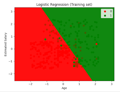
# Visualising the Training set results
from matplotlib.colors import ListedColormap
X_set, y_set = X_train, y_train
X1, X2 = np.meshgrid(np.arange(start = X_set[:, 0].min() - 1, stop = X_set[:, 0].max() + 1, step = 0.01),
np.arange(start = X_set[:, 1].min() - 1, stop = X_set[:, 1].max() + 1, step = 0.01))
plt.contourf(X1, X2, classifier.predict(np.array([X1.ravel(), X2.ravel()]).T).reshape(X1.shape),
alpha = 0.75, cmap = ListedColormap(('red', 'green')))
plt.xlim(X1.min(), X1.max())
plt.ylim(X2.min(), X2.max())
for i, j in enumerate(np.unique(y_set)):
plt.scatter(X_set[y_set == j, 0], X_set[y_set == j, 1],
c = ListedColormap(('red', 'green'))(i), label = j)
plt.title('Logistic Regression (Training set)')
plt.xlabel('Age')
plt.ylabel('Estimated Salary')
plt.legend()
plt.show()
# Visualising the Test set results
from matplotlib.colors import ListedColormap
X_set, y_set = X_test, y_test
X1, X2 = np.meshgrid(np.arange(start = X_set[:, 0].min() - 1, stop = X_set[:, 0].max() + 1, step = 0.01),
np.arange(start = X_set[:, 1].min() - 1, stop = X_set[:, 1].max() + 1, step = 0.01))
plt.contourf(X1, X2, classifier.predict(np.array([X1.ravel(), X2.ravel()]).T).reshape(X1.shape),
alpha = 0.75, cmap = ListedColormap(('red', 'green')))
plt.xlim(X1.min(), X1.max())
plt.ylim(X2.min(), X2.max())
for i, j in enumerate(np.unique(y_set)):
plt.scatter(X_set[y_set == j, 0], X_set[y_set == j, 1],
c = ListedColormap(('red', 'green'))(i), label = j)
plt.title('Logistic Regression (Test set)')
plt.xlabel('Age')
plt.ylabel('Estimated Salary')
plt.legend()
plt.show()

Hope this helps!!!.
Arun Manglick
In statistics, logistic regression, is a regression model where the dependent variable (DV) is Categorical. I.e. where there is a binary dependent variable—that is, where it can take only two values, "0" and "1", which represent outcomes such as pass/fail, win/lose, alive/dead or healthy/sick.
E.g At a certain age, people will buy parachute or not. This problem is not a linear problem. It's either be Yes or No (Categorical Problem). Such problems are resolved thru Logistic Regression.
E.g. A group of 20 students spend between 0 and 6 hours studying for an exam. How does the number of hours spent studying affect the probability that the student will pass the exam?
Ans: The reason for using logistic regression for this problem is that the dependent variable pass/fail represented by "1" and "0" are not cardinal numbers. If the problem was changed so that pass/fail was replaced with the grade 0–100 (cardinal numbers), then simple regression analysis could be used.

In summary, Logistic Regression is used to estimate the Probability (0-1) of a binary response based on one or more predictor (or independent) variables (features).


The above shows how linear regression is used to deduce Logistic Regression formula, using Sigmoid Function.
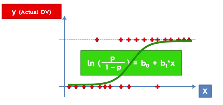

Based on above, probability model, it can be deduced that predicted values for probability less than 50% would be close to 0 and for above 50% close to 1.

Code: # Logistic Regression
# Importing the libraries
import numpy as np
import matplotlib.pyplot as plt
import pandas as pd
# Importing the dataset
dataset = pd.read_csv('Social_Network_Ads.csv')
X = dataset.iloc[:, [2, 3]].values
y = dataset.iloc[:, 4].values
# Splitting the dataset into the Training set and Test set
from sklearn.cross_validation import train_test_split
X_train, X_test, y_train, y_test = train_test_split(X, y, test_size = 0.25, random_state = 0)
# Feature Scaling
from sklearn.preprocessing import StandardScaler
sc = StandardScaler()
X_train = sc.fit_transform(X_train)
X_test = sc.transform(X_test)
# Fitting Logistic Regression to the Training set
from sklearn.linear_model import LogisticRegression
classifier = LogisticRegression(random_state = 0)
classifier.fit(X_train, y_train)
# Predicting the Test set results
y_pred = classifier.predict(X_test)
# Making the Confusion Matrix
# Used to evauate performance of model to see corret/incorrection predictions made by Logistic regression
from sklearn.metrics import confusion_matrix
cm = confusion_matrix(y_test, y_pred)
# Visualising the Training set results
from matplotlib.colors import ListedColormap
X_set, y_set = X_train, y_train
X1, X2 = np.meshgrid(np.arange(start = X_set[:, 0].min() - 1, stop = X_set[:, 0].max() + 1, step = 0.01),
np.arange(start = X_set[:, 1].min() - 1, stop = X_set[:, 1].max() + 1, step = 0.01))
plt.contourf(X1, X2, classifier.predict(np.array([X1.ravel(), X2.ravel()]).T).reshape(X1.shape),
alpha = 0.75, cmap = ListedColormap(('red', 'green')))
plt.xlim(X1.min(), X1.max())
plt.ylim(X2.min(), X2.max())
for i, j in enumerate(np.unique(y_set)):
plt.scatter(X_set[y_set == j, 0], X_set[y_set == j, 1],
c = ListedColormap(('red', 'green'))(i), label = j)
plt.title('Logistic Regression (Training set)')
plt.xlabel('Age')
plt.ylabel('Estimated Salary')
plt.legend()
plt.show()

# Visualising the Test set results
from matplotlib.colors import ListedColormap
X_set, y_set = X_test, y_test
X1, X2 = np.meshgrid(np.arange(start = X_set[:, 0].min() - 1, stop = X_set[:, 0].max() + 1, step = 0.01),
np.arange(start = X_set[:, 1].min() - 1, stop = X_set[:, 1].max() + 1, step = 0.01))
plt.contourf(X1, X2, classifier.predict(np.array([X1.ravel(), X2.ravel()]).T).reshape(X1.shape),
alpha = 0.75, cmap = ListedColormap(('red', 'green')))
plt.xlim(X1.min(), X1.max())
plt.ylim(X2.min(), X2.max())
for i, j in enumerate(np.unique(y_set)):
plt.scatter(X_set[y_set == j, 0], X_set[y_set == j, 1],
c = ListedColormap(('red', 'green'))(i), label = j)
plt.title('Logistic Regression (Test set)')
plt.xlabel('Age')
plt.ylabel('Estimated Salary')
plt.legend()
plt.show()

Hope this helps!!!.
Arun Manglick
No comments:
Post a Comment