Basics:
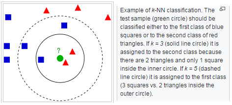
In pattern recognition, the k-nearest neighbors algorithm (k-NN) is a non-parametric method used for Classification and Regression. In both cases, the input consists of the k closest training examples in the feature space. The output depends on whether k-NN is used for classification or regression:
Both for classification and regression, it can be useful to assign weight to the contributions of the neighbors, so that the nearer neighbors contribute more to the average than the more distant ones.For example, a common weighting scheme consists in giving each neighbor a weight of 1/d, where d is the distance to the neighbor.


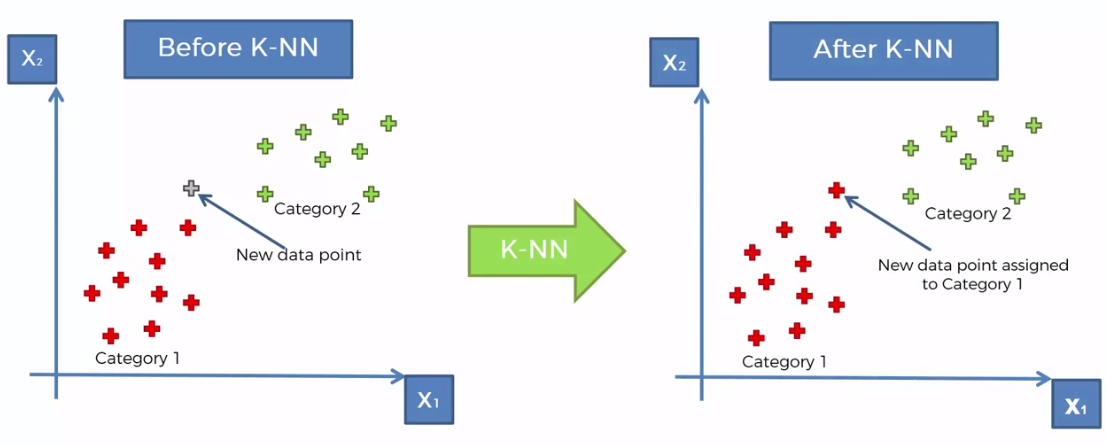
One more example:
Code: K-Nearest Neighbors (K-NN)
# Importing the libraries
import numpy as np
import matplotlib.pyplot as plt
import pandas as pd
# Importing the dataset
dataset = pd.read_csv('Social_Network_Ads.csv')
X = dataset.iloc[:, [2, 3]].values
y = dataset.iloc[:, 4].values
# Splitting the dataset into the Training set and Test set
from sklearn.cross_validation import train_test_split
X_train, X_test, y_train, y_test = train_test_split(X, y, test_size = 0.25, random_state = 0)
# Feature Scaling
from sklearn.preprocessing import StandardScaler
sc = StandardScaler()
X_train = sc.fit_transform(X_train)
X_test = sc.transform(X_test)
# Fitting K-NN to the Training set
from sklearn.neighbors import KNeighborsClassifier
classifier = KNeighborsClassifier(n_neighbors = 5, metric = 'minkowski', p = 2)
classifier.fit(X_train, y_train)
# Predicting the Test set results
y_pred = classifier.predict(X_test)
# Making the Confusion Matrix
from sklearn.metrics import confusion_matrix
cm = confusion_matrix(y_test, y_pred)
# Visualising the Training set results
from matplotlib.colors import ListedColormap
X_set, y_set = X_train, y_train
X1, X2 = np.meshgrid(np.arange(start = X_set[:, 0].min() - 1, stop = X_set[:, 0].max() + 1, step = 0.01),
np.arange(start = X_set[:, 1].min() - 1, stop = X_set[:, 1].max() + 1, step = 0.01))
plt.contourf(X1, X2, classifier.predict(np.array([X1.ravel(), X2.ravel()]).T).reshape(X1.shape),
alpha = 0.75, cmap = ListedColormap(('red', 'green')))
plt.xlim(X1.min(), X1.max())
plt.ylim(X2.min(), X2.max())
for i, j in enumerate(np.unique(y_set)):
plt.scatter(X_set[y_set == j, 0], X_set[y_set == j, 1],
c = ListedColormap(('red', 'green'))(i), label = j)
plt.title('K-NN (Training set)')
plt.xlabel('Age')
plt.ylabel('Estimated Salary')
plt.legend()
plt.show()

# Visualising the Test set results
from matplotlib.colors import ListedColormap
X_set, y_set = X_test, y_test
X1, X2 = np.meshgrid(np.arange(start = X_set[:, 0].min() - 1, stop = X_set[:, 0].max() + 1, step = 0.01),
np.arange(start = X_set[:, 1].min() - 1, stop = X_set[:, 1].max() + 1, step = 0.01))
plt.contourf(X1, X2, classifier.predict(np.array([X1.ravel(), X2.ravel()]).T).reshape(X1.shape),
alpha = 0.75, cmap = ListedColormap(('red', 'green')))
plt.xlim(X1.min(), X1.max())
plt.ylim(X2.min(), X2.max())
for i, j in enumerate(np.unique(y_set)):
plt.scatter(X_set[y_set == j, 0], X_set[y_set == j, 1],
c = ListedColormap(('red', 'green'))(i), label = j)
plt.title('K-NN (Test set)')
plt.xlabel('Age')
plt.ylabel('Estimated Salary')
plt.legend()
plt.show()

Hope this helps.
Arun Manglick
In pattern recognition, the k-nearest neighbors algorithm (k-NN) is a non-parametric method used for Classification and Regression. In both cases, the input consists of the k closest training examples in the feature space. The output depends on whether k-NN is used for classification or regression:
- In k-NN classification, the output is a class membership. An object is classified by a majority vote of its neighbors, with the object being assigned to the class most common among its k nearest neighbors (k is a positive integer, typically small). If k = 1, then the object is simply assigned to the class of that single nearest neighbor.
- In k-NN regression, the output is the property value for the object. This value is the average of the values of its k nearest neighbors.
Both for classification and regression, it can be useful to assign weight to the contributions of the neighbors, so that the nearer neighbors contribute more to the average than the more distant ones.For example, a common weighting scheme consists in giving each neighbor a weight of 1/d, where d is the distance to the neighbor.


Code: K-Nearest Neighbors (K-NN)
# Importing the libraries
import numpy as np
import matplotlib.pyplot as plt
import pandas as pd
# Importing the dataset
dataset = pd.read_csv('Social_Network_Ads.csv')
X = dataset.iloc[:, [2, 3]].values
y = dataset.iloc[:, 4].values
# Splitting the dataset into the Training set and Test set
from sklearn.cross_validation import train_test_split
X_train, X_test, y_train, y_test = train_test_split(X, y, test_size = 0.25, random_state = 0)
# Feature Scaling
from sklearn.preprocessing import StandardScaler
sc = StandardScaler()
X_train = sc.fit_transform(X_train)
X_test = sc.transform(X_test)
# Fitting K-NN to the Training set
from sklearn.neighbors import KNeighborsClassifier
classifier = KNeighborsClassifier(n_neighbors = 5, metric = 'minkowski', p = 2)
classifier.fit(X_train, y_train)
# Predicting the Test set results
y_pred = classifier.predict(X_test)
# Making the Confusion Matrix
from sklearn.metrics import confusion_matrix
cm = confusion_matrix(y_test, y_pred)
# Visualising the Training set results
from matplotlib.colors import ListedColormap
X_set, y_set = X_train, y_train
X1, X2 = np.meshgrid(np.arange(start = X_set[:, 0].min() - 1, stop = X_set[:, 0].max() + 1, step = 0.01),
np.arange(start = X_set[:, 1].min() - 1, stop = X_set[:, 1].max() + 1, step = 0.01))
plt.contourf(X1, X2, classifier.predict(np.array([X1.ravel(), X2.ravel()]).T).reshape(X1.shape),
alpha = 0.75, cmap = ListedColormap(('red', 'green')))
plt.xlim(X1.min(), X1.max())
plt.ylim(X2.min(), X2.max())
for i, j in enumerate(np.unique(y_set)):
plt.scatter(X_set[y_set == j, 0], X_set[y_set == j, 1],
c = ListedColormap(('red', 'green'))(i), label = j)
plt.title('K-NN (Training set)')
plt.xlabel('Age')
plt.ylabel('Estimated Salary')
plt.legend()
plt.show()

from matplotlib.colors import ListedColormap
X_set, y_set = X_test, y_test
X1, X2 = np.meshgrid(np.arange(start = X_set[:, 0].min() - 1, stop = X_set[:, 0].max() + 1, step = 0.01),
np.arange(start = X_set[:, 1].min() - 1, stop = X_set[:, 1].max() + 1, step = 0.01))
plt.contourf(X1, X2, classifier.predict(np.array([X1.ravel(), X2.ravel()]).T).reshape(X1.shape),
alpha = 0.75, cmap = ListedColormap(('red', 'green')))
plt.xlim(X1.min(), X1.max())
plt.ylim(X2.min(), X2.max())
for i, j in enumerate(np.unique(y_set)):
plt.scatter(X_set[y_set == j, 0], X_set[y_set == j, 1],
c = ListedColormap(('red', 'green'))(i), label = j)
plt.title('K-NN (Test set)')
plt.xlabel('Age')
plt.ylabel('Estimated Salary')
plt.legend()
plt.show()

Hope this helps.
Arun Manglick
No comments:
Post a Comment