XGBoost

Basics:

XGBoost stands for eXtreme Gradient Boosting. It's an implementation of gradient boosted decision trees designed for Speed and Performance.

Three main forms of Gradient Boosting are supported:

1. Gradient Boosting algorithm also called gradient boosting machine including the learning rate.
2. Stochastic Gradient Boosting with sub-sampling at the row, column and column per split levels.
3. Regularized Gradient Boosting with both L1 and L2 regularization

XGBoost is an algorithm that has recently been dominating applied machine learning and Kaggle competitions for structured or tabular data.

XGBoost is a software library that you can download and install on your machine, then access from a variety of interfaces. Specifically, XGBoost supports the following main interfaces:

• Command Line Interface (CLI).
• C++ (the language in which the library is written).
• Python interface as well as a model in scikit-learn.
• R interface as well as a model in the caret package.
• Julia.
• Java and JVM languages like Scala and platforms like Hadoop.

It belongs to a broader collection of tools under the umbrella of the Distributed Machine Learning Community or DMLC who are also the creators of the popular mxnet deep learning library.

Installation Guide - http://xgboost.readthedocs.io/en/latest/build.html#

Business Problem: (Same as used in ANN)
You have bank customers (credit score, country, age, gender, tenure,balance, credit card, loan, exited etc). Given the problem you need to find out which customers are at high risk of leaving the bank.
In summary, it's a Classification Problem.

Code: XGBoost

# Importing the libraries
import numpy as np
import matplotlib.pyplot as plt
import pandas as pd

# Importing the dataset
dataset = pd.read_csv('Churn_Modelling.csv')
X = dataset.iloc[:, 3:13].values
y = dataset.iloc[:, 13].values

# Encoding categorical data
from sklearn.preprocessing import LabelEncoder, OneHotEncoder
labelencoder_X_1 = LabelEncoder()
X[:, 1] = labelencoder_X_1.fit_transform(X[:, 1])
labelencoder_X_2 = LabelEncoder()
X[:, 2] = labelencoder_X_2.fit_transform(X[:, 2])
onehotencoder = OneHotEncoder(categorical_features = [1])
X = onehotencoder.fit_transform(X).toarray()
X = X[:, 1:]

# Splitting the dataset into the Training set and Test set
from sklearn.model_selection import train_test_split
X_train, X_test, y_train, y_test = train_test_split(X, y, test_size = 0.2, random_state = 0)

# Fitting XGBoost to the Training set
from xgboost import XGBClassifier
classifier = XGBClassifier()
classifier.fit(X_train, y_train)

# Predicting the Test set results
y_pred = classifier.predict(X_test)

# Making the Confusion Matrix
from sklearn.metrics import confusion_matrix
cm = confusion_matrix(y_test, y_pred)

# Applying k-Fold Cross Validation
from sklearn.model_selection import cross_val_score
accuracies = cross_val_score(estimator = classifier, X = X_train, y = y_train, cv = 10)
accuracies.mean()
accuracies.std()


Hope this helps!!

Arun Manglick

Model Selection

1). k-fold cross-validation:

In k-fold cross-validation, the original sample is randomly partitioned into k equal sized sub-samples. Of the k sub-samples:

• Single sub-sample is retained as the validation data for testing the model, and 
• Remaining k − 1 sub-samples are used as training data. 

The cross-validation process is then repeated k times (the folds), with each of the k subsamples used exactly once as the validation data. The k results from the folds can then be averaged to produce a single estimation. The advantage of this method over repeated random sub-sampling (see below) is that all observations are used for both training and validation, and each observation is used for validation exactly once. 10-fold cross-validation is commonly used,[7] but in general k remains an unfixed parameter.

For example, setting k = 2 results in 2-fold cross-validation. In 2-fold cross-validation, we randomly shuffle the dataset into two sets d0 and d1, so that both sets are equal size (this is usually implemented by shuffling the data array and then splitting it in two). We then train on d0 and test on d1, followed by training on d1 and testing on d0.

When k = n (the number of observations), the k-fold cross-validation is exactly the leave-one-out cross-validation.

In stratified k-fold cross-validation, the folds are selected so that the mean response value is approximately equal in all the folds. In the case of a dichotomous classification, this means that each fold contains roughly the same proportions of the two types of class labels.

Business Problem: 

Problem is taken from Classification examples (Part 3 - Kernel SVM), where given a set of male/female with a age and salary, will click on a advertisement or not.

Code: k-Fold Cross Validation

# Importing the libraries
import numpy as np
import matplotlib.pyplot as plt
import pandas as pd

# Importing the dataset
dataset = pd.read_csv('Social_Network_Ads.csv')
X = dataset.iloc[:, [2, 3]].values
y = dataset.iloc[:, 4].values

# Splitting the dataset into the Training set and Test set
from sklearn.model_selection import train_test_split
X_train, X_test, y_train, y_test = train_test_split(X, y, test_size = 0.25, random_state = 0)

# Feature Scaling
from sklearn.preprocessing import StandardScaler
sc = StandardScaler()
X_train = sc.fit_transform(X_train)
X_test = sc.transform(X_test)

# Fitting Kernel SVM to the Training set - (Part 3 - Kernel SVM),
from sklearn.svm import SVC
classifier = SVC(kernel = 'rbf', random_state = 0)
classifier.fit(X_train, y_train)

# Predicting the Test set results
y_pred = classifier.predict(X_test)

# Making the Confusion Matrix
# Used to evauate performance of model to see corret/incorrection predictions made by Logistic regression
from sklearn.metrics import confusion_matrix
cm = confusion_matrix(y_test, y_pred)

# Applying k-Fold Cross Validation
from sklearn.model_selection import cross_val_score
accuracies = cross_val_score(estimator = classifier, X = X_train, y = y_train, cv = 10)
accuracies.mean()
accuracies.std()

# Visualising the Training set results
from matplotlib.colors import ListedColormap
X_set, y_set = X_train, y_train
X1, X2 = np.meshgrid(np.arange(start = X_set[:, 0].min() - 1, stop = X_set[:, 0].max() + 1, step = 0.01),
                     np.arange(start = X_set[:, 1].min() - 1, stop = X_set[:, 1].max() + 1, step = 0.01))
plt.contourf(X1, X2, classifier.predict(np.array([X1.ravel(), X2.ravel()]).T).reshape(X1.shape),
             alpha = 0.75, cmap = ListedColormap(('red', 'green')))
plt.xlim(X1.min(), X1.max())
plt.ylim(X2.min(), X2.max())
for i, j in enumerate(np.unique(y_set)):
    plt.scatter(X_set[y_set == j, 0], X_set[y_set == j, 1],
                c = ListedColormap(('red', 'green'))(i), label = j)
plt.title('Kernel SVM (Training set)')
plt.xlabel('Age')
plt.ylabel('Estimated Salary')
plt.legend()
plt.show()

# Visualising the Test set results
from matplotlib.colors import ListedColormap
X_set, y_set = X_test, y_test
X1, X2 = np.meshgrid(np.arange(start = X_set[:, 0].min() - 1, stop = X_set[:, 0].max() + 1, step = 0.01),
                     np.arange(start = X_set[:, 1].min() - 1, stop = X_set[:, 1].max() + 1, step = 0.01))
plt.contourf(X1, X2, classifier.predict(np.array([X1.ravel(), X2.ravel()]).T).reshape(X1.shape),
             alpha = 0.75, cmap = ListedColormap(('red', 'green')))
plt.xlim(X1.min(), X1.max())
plt.ylim(X2.min(), X2.max())
for i, j in enumerate(np.unique(y_set)):
    plt.scatter(X_set[y_set == j, 0], X_set[y_set == j, 1],
                c = ListedColormap(('red', 'green'))(i), label = j)
plt.title('Kernel SVM (Test set)')
plt.xlabel('Age')
plt.ylabel('Estimated Salary')
plt.legend()
plt.show()

2).Grid Search:

This method is used to - Improve model performance by choosing the optimal values for the Hyper-parameters (the parameters that are not learned).

Hyper-parameters are parameters that are not directly learnt within estimators. In scikit-learn they are passed as arguments to the constructor of the estimator classes. Typical examples include C, kernel and gamma for Support Vector Classifier, alpha for Lasso, etc

Any parameter provided when constructing an estimator may be optimized in this manner. Specifically, to find the names and current values for all parameters for a given estimator, use:
estimator.get_params()

A search consists of:

• an estimator (regressor or classifier such as sklearn.svm.SVC());
• a parameter space;
• a method for searching or sampling candidates;
• a cross-validation scheme; and
• a score function.

Two generic approaches to sampling search candidates are provided in scikit-learn: for given values,

• GridSearchCV exhaustively considers all parameter combinations, while 
• RandomizedSearchCV can sample a given number of candidates from a parameter space with a specified distribution.

The GridSearchCV instance implements the usual estimator API: when “fitting” it on a dataset all the possible combinations of parameter values are evaluated and the best combination is retained.

Note: A small subset of those parameters can have a large impact on the predictive or computation performance of the model while others can be left to their default value.

The grid search provided by GridSearchCV exhaustively generates candidates from a grid of parameter values specified with the param_grid parameter. For instance, the following param_grid:

param_grid = [
  {'C': [1, 10, 100, 1000], 'kernel': ['linear']},
  {'C': [1, 10, 100, 1000], 'gamma': [0.001, 0.0001], 'kernel': ['rbf']},
 ]

specifies that two grids should be explored:

• one with a Linear kernel and C values in [1, 10, 100, 1000], and  
• second one with an RBF kernel, and the cross-product of C values ranging in [1, 10, 100, 1000] and gamma values in [0.001, 0.0001].

Business Problem: 

Problem is taken from Classification examples (Part 3 - Kernel SVM), where given a set of male/female with a age and salary, will click on a advertisement or not.

Code: Grid Search

# Importing the libraries
import numpy as np
import matplotlib.pyplot as plt
import pandas as pd

# Importing the dataset
dataset = pd.read_csv('Social_Network_Ads.csv')
X = dataset.iloc[:, [2, 3]].values
y = dataset.iloc[:, 4].values

# Splitting the dataset into the Training set and Test set
from sklearn.model_selection import train_test_split
X_train, X_test, y_train, y_test = train_test_split(X, y, test_size = 0.25, random_state = 0)

# Feature Scaling
from sklearn.preprocessing import StandardScaler
sc = StandardScaler()
X_train = sc.fit_transform(X_train)
X_test = sc.transform(X_test)

# Fitting Kernel SVM to the Training set
from sklearn.svm import SVC
classifier = SVC(kernel = 'rbf', random_state = 0)
classifier.fit(X_train, y_train)

# Predicting the Test set results
y_pred = classifier.predict(X_test)

# Making the Confusion Matrix
from sklearn.metrics import confusion_matrix
cm = confusion_matrix(y_test, y_pred)

# Applying k-Fold Cross Validation
from sklearn.model_selection import cross_val_score
accuracies = cross_val_score(estimator = classifier, X = X_train, y = y_train, cv = 10)
accuracies.mean()
accuracies.std()

# Applying Grid Search to find the best model and the best parameters
# Applying Grid Search to find the best model (Linear/Non-Linear (rbf)) and the best parameters
# C - Penalty Parameter

# kernel - Kernel Type (Linear, poly, rbf, sigmoid, precomputed, callable)
from sklearn.model_selection import GridSearchCV
parameters = [
              {'C': [1, 10, 100, 1000], 'kernel': ['linear']},
              {'C': [1, 10, 100, 1000], 'kernel': ['rbf'], 'gamma': [0.1, 0.2, 0.3, 0.4, 0.5, 0.6, 0.7, 0.8, 0.9]}
             ]

grid_search = GridSearchCV(estimator = classifier,
                           param_grid = parameters,
                           scoring = 'accuracy',
                           cv = 10,
                           n_jobs = -1)

grid_search = grid_search.fit(X_train, y_train)
best_accuracy = grid_search.best_score_
best_parameters = grid_search.best_params_   # Here output says 'Non-Linear' model will be the best suitable for the given problem.

# Visualising the Training set results (Optional Here)
from matplotlib.colors import ListedColormap
X_set, y_set = X_train, y_train
X1, X2 = np.meshgrid(np.arange(start = X_set[:, 0].min() - 1, stop = X_set[:, 0].max() + 1, step = 0.01),
                     np.arange(start = X_set[:, 1].min() - 1, stop = X_set[:, 1].max() + 1, step = 0.01))
plt.contourf(X1, X2, classifier.predict(np.array([X1.ravel(), X2.ravel()]).T).reshape(X1.shape),
             alpha = 0.75, cmap = ListedColormap(('red', 'green')))
plt.xlim(X1.min(), X1.max())
plt.ylim(X2.min(), X2.max())
for i, j in enumerate(np.unique(y_set)):
    plt.scatter(X_set[y_set == j, 0], X_set[y_set == j, 1],
                c = ListedColormap(('red', 'green'))(i), label = j)
plt.title('Kernel SVM (Training set)')
plt.xlabel('Age')
plt.ylabel('Estimated Salary')
plt.legend()
plt.show()

# Visualising the Test set results  (Optional Here)
from matplotlib.colors import ListedColormap
X_set, y_set = X_test, y_test
X1, X2 = np.meshgrid(np.arange(start = X_set[:, 0].min() - 1, stop = X_set[:, 0].max() + 1, step = 0.01),
                     np.arange(start = X_set[:, 1].min() - 1, stop = X_set[:, 1].max() + 1, step = 0.01))
plt.contourf(X1, X2, classifier.predict(np.array([X1.ravel(), X2.ravel()]).T).reshape(X1.shape),
             alpha = 0.75, cmap = ListedColormap(('red', 'green')))
plt.xlim(X1.min(), X1.max())
plt.ylim(X2.min(), X2.max())
for i, j in enumerate(np.unique(y_set)):
    plt.scatter(X_set[y_set == j, 0], X_set[y_set == j, 1],
                c = ListedColormap(('red', 'green'))(i), label = j)
plt.title('Kernel SVM (Test set)')
plt.xlabel('Age')
plt.ylabel('Estimated Salary')
plt.legend()
plt.show()

Hope this helps.

Arun Manglick

Part 10: Model Selection & Boosting

Here we'll try to address few questions using Model Selection techniques.

• How to find the most appropriate Machine Learning model for my business problem ?
• How to deal with the bias variance tradeoff when building a model and evaluating its performance - k-Fold Cross Validation 
• How to Improve model performance by choosing the optimal values for the hyper-parameters (the parameters that are not learned) -  Grid Search

Model Selection techniques are:

• k-Fold Cross Validation - Used to Evaluate Model Performance
• Grid Search - Use to Improve Model Performance (Finding optimal values for the hyper-parameters)

In last we'll learn the most powerful Machine Learning model: XGBoost.

Cheat Sheet: 

For a given dataset, First step is to know business problem.

• Regression (Have Dependent Variable & Continuous Outcome)
• Classification (Have Dependent Variable & Categorical Outcome)
• Clustering (No Dependent Variable)

Second step is to know problem is Linear/Non-Linear Separable. E.g Choose SVM (For Linear) and Kernel SVM for Non-Linear. To know this question, Grid Search is the best method.

Hope this helps!!

Arun Manglick

Kernel PCA

Basics:

In the field of multivariate statistics, Kernel Principal Component Analysis (kernel PCA) is an extension of principal component analysis (PCA) using techniques of kernel methods. Using a kernel, the originally linear operations of PCA are performed in a reproducing Kernel Hilbert space.

Business Problem: 

Problem is taken from Classification examples (Part 3 - Kernel SVM), where given a set of male/female with a age and salary, will click on a advertisement or not.

Code: # Kernel PCA

# Importing the libraries
import numpy as np
import matplotlib.pyplot as plt
import pandas as pd

# Importing the dataset
dataset = pd.read_csv('Social_Network_Ads.csv')
X = dataset.iloc[:, [2, 3]].values
y = dataset.iloc[:, 4].values

# Splitting the dataset into the Training set and Test set
from sklearn.model_selection import train_test_split
X_train, X_test, y_train, y_test = train_test_split(X, y, test_size = 0.25, random_state = 0)

# Feature Scaling
from sklearn.preprocessing import StandardScaler
sc = StandardScaler()
X_train = sc.fit_transform(X_train)
X_test = sc.transform(X_test)

# Applying Kernel PCA
from sklearn.decomposition import KernelPCA
# rbf is 'Gaussian Kernel'
kpca = KernelPCA(n_components = 2, kernel = 'rbf')
X_train = kpca.fit_transform(X_train)
X_test = kpca.transform(X_test)

# Fitting Logistic Regression to the Training set
from sklearn.linear_model import LogisticRegression
classifier = LogisticRegression(random_state = 0)
classifier.fit(X_train, y_train)

# Predicting the Test set results
y_pred = classifier.predict(X_test)

# Making the Confusion Matrix
# Used to evauate performance of model to see corret/incorrection predictions made by Logistic regression
from sklearn.metrics import confusion_matrix
cm = confusion_matrix(y_test, y_pred)

# Visualising the Training set results
from matplotlib.colors import ListedColormap
X_set, y_set = X_train, y_train
X1, X2 = np.meshgrid(np.arange(start = X_set[:, 0].min() - 1, stop = X_set[:, 0].max() + 1, step = 0.01),
                     np.arange(start = X_set[:, 1].min() - 1, stop = X_set[:, 1].max() + 1, step = 0.01))
plt.contourf(X1, X2, classifier.predict(np.array([X1.ravel(), X2.ravel()]).T).reshape(X1.shape),
             alpha = 0.75, cmap = ListedColormap(('red', 'green')))
plt.xlim(X1.min(), X1.max())
plt.ylim(X2.min(), X2.max())
for i, j in enumerate(np.unique(y_set)):
    plt.scatter(X_set[y_set == j, 0], X_set[y_set == j, 1],
                c = ListedColormap(('red', 'green'))(i), label = j)
plt.title('Logistic Regression (Training set)')
plt.xlabel('Age')
plt.ylabel('Estimated Salary')
plt.legend()
plt.show()

# Visualising the Test set results
from matplotlib.colors import ListedColormap
X_set, y_set = X_test, y_test
X1, X2 = np.meshgrid(np.arange(start = X_set[:, 0].min() - 1, stop = X_set[:, 0].max() + 1, step = 0.01),
                     np.arange(start = X_set[:, 1].min() - 1, stop = X_set[:, 1].max() + 1, step = 0.01))
plt.contourf(X1, X2, classifier.predict(np.array([X1.ravel(), X2.ravel()]).T).reshape(X1.shape),
             alpha = 0.75, cmap = ListedColormap(('red', 'green')))
plt.xlim(X1.min(), X1.max())
plt.ylim(X2.min(), X2.max())
for i, j in enumerate(np.unique(y_set)):
    plt.scatter(X_set[y_set == j, 0], X_set[y_set == j, 1],
                c = ListedColormap(('red', 'green'))(i), label = j)
plt.title('Logistic Regression (Test set)')
plt.xlabel('Age')
plt.ylabel('Estimated Salary')
plt.legend()
plt.show()

Hope this helps!!

Arun Manglick

Linear Discriminant Analysis (LDA)

Basics:

From m independent variables of given dataset, LDA extracts p <= m new independent variables that separate most of the classes of the dependent variables.

Linear discriminant analysis (LDA) is a generalization of Fisher's linear discriminant, a method used in statistics, pattern recognition and machine learning to find a linear combination of features that characterizes or separates two or more classes of objects or events.

LDA is also closely related to PCA in that they both look for linear combinations of variables which best explain the data.

• LDA explicitly attempts to model the difference between the classes of data. 
• PCA on the other hand does not take into account any difference in class

Business Problem: 

(Same as in PCA) Given 13 independent variables (various type of alcohol) in wine, decide which customer segment will prefer a particular type of wine. Now as it's tough to determine customer segment on bases of so many independent variables, we'll apply PCA and deduce best two  independent variables to solve this problem.

Code: LDA

# Importing the libraries
import numpy as np
import matplotlib.pyplot as plt
import pandas as pd

# Importing the dataset
dataset = pd.read_csv('Wine.csv')
X = dataset.iloc[:, 0:13].values
y = dataset.iloc[:, 13].values

# Splitting the dataset into the Training set and Test set
from sklearn.model_selection import train_test_split
X_train, X_test, y_train, y_test = train_test_split(X, y, test_size = 0.2, random_state = 0)

# Feature Scaling
from sklearn.preprocessing import StandardScaler
sc = StandardScaler()
X_train = sc.fit_transform(X_train)
X_test = sc.transform(X_test)

# Applying LDA
from sklearn.discriminant_analysis import LinearDiscriminantAnalysis as LDA
lda = LDA(n_components = 2)
X_train = lda.fit_transform(X_train, y_train)  # This is additional here in comparison to LCA
X_test = lda.transform(X_test)

# Fitting Logistic Regression to the Training set
from sklearn.linear_model import LogisticRegression
classifier = LogisticRegression(random_state = 0)
classifier.fit(X_train, y_train)

# Predicting the Test set results
y_pred = classifier.predict(X_test)

# Making the Confusion Matrix
# Used to evauate performance of model to see corret/incorrection predictions made by Logistic regression
from sklearn.metrics import confusion_matrix
cm = confusion_matrix(y_test, y_pred)

# Visualising the Training set results
from matplotlib.colors import ListedColormap
X_set, y_set = X_train, y_train
X1, X2 = np.meshgrid(np.arange(start = X_set[:, 0].min() - 1, stop = X_set[:, 0].max() + 1, step = 0.01),
                     np.arange(start = X_set[:, 1].min() - 1, stop = X_set[:, 1].max() + 1, step = 0.01))
plt.contourf(X1, X2, classifier.predict(np.array([X1.ravel(), X2.ravel()]).T).reshape(X1.shape),
             alpha = 0.75, cmap = ListedColormap(('red', 'green', 'blue')))
plt.xlim(X1.min(), X1.max())
plt.ylim(X2.min(), X2.max())
for i, j in enumerate(np.unique(y_set)):
    plt.scatter(X_set[y_set == j, 0], X_set[y_set == j, 1],
                c = ListedColormap(('red', 'green', 'blue'))(i), label = j)
plt.title('Logistic Regression (Training set)')
plt.xlabel('LD1')
plt.ylabel('LD2')
plt.legend()
plt.show()

# Visualising the Test set results
from matplotlib.colors import ListedColormap
X_set, y_set = X_test, y_test
X1, X2 = np.meshgrid(np.arange(start = X_set[:, 0].min() - 1, stop = X_set[:, 0].max() + 1, step = 0.01),
                     np.arange(start = X_set[:, 1].min() - 1, stop = X_set[:, 1].max() + 1, step = 0.01))
plt.contourf(X1, X2, classifier.predict(np.array([X1.ravel(), X2.ravel()]).T).reshape(X1.shape),
             alpha = 0.75, cmap = ListedColormap(('red', 'green', 'blue')))
plt.xlim(X1.min(), X1.max())
plt.ylim(X2.min(), X2.max())
for i, j in enumerate(np.unique(y_set)):
    plt.scatter(X_set[y_set == j, 0], X_set[y_set == j, 1],
                c = ListedColormap(('red', 'green', 'blue'))(i), label = j)
plt.title('Logistic Regression (Test set)')
plt.xlabel('LD1')
plt.ylabel('LD2')
plt.legend()
plt.show()

Hope this helps!!

Arun Manglick

Principal Component Analysis (PCA)

Basics:

From m independent variables of given dataset, PCA extracts p <= m new independent variables that explain most of the variance of the dataset, regardless of the dependent variables.

Principal component analysis (PCA) is a statistical procedure that uses an orthogonal transformation to convert a set of observations of possibly correlated variables into a set of values of linearly uncorrelated variables called Principal Components (or sometimes, principal modes of variation).

The number of principal components is less than or equal to the smaller of the number of original variables or the number of observations.

This transformation is defined in such a way that the first principal component has the largest possible variance (that is, accounts for as much of the variability in the data as possible), and each succeeding component in turn has the highest variance possible under the constraint that it is orthogonal to the preceding components. The resulting vectors are an uncorrelated orthogonal basis set. PCA is sensitive to the relative scaling of the original variables.

Business Problem: 

Given 13 independent variables (various type of alcohol) in wine, decide which customer segment will prefer a particular type of wine. Now as it's tough to determine customer segment on bases of so many independent variables, we'll apply PCA and deduce best two  independent variables to solve this problem.

Code: PCA

# Importing the libraries
import numpy as np
import matplotlib.pyplot as plt
import pandas as pd

# Importing the dataset
dataset = pd.read_csv('Wine.csv')
X = dataset.iloc[:, 0:13].values
y = dataset.iloc[:, 13].values

# Splitting the dataset into the Training set and Test set
from sklearn.model_selection import train_test_split
X_train, X_test, y_train, y_test = train_test_split(X, y, test_size = 0.2, random_state = 0)

# Feature Scaling
from sklearn.preprocessing import StandardScaler
sc = StandardScaler()
X_train = sc.fit_transform(X_train)
X_test = sc.transform(X_test)

# Applying PCA
from sklearn.decomposition import PCA
# It extracts two principal component variables which has largest variance.
pca = PCA(n_components = 2)  
X_train = pca.fit_transform(X_train)
X_test = pca.transform(X_test)
explained_variance = pca.explained_variance_ratio_

# Fitting Logistic Regression to the Training set
from sklearn.linear_model import LogisticRegression
classifier = LogisticRegression(random_state = 0)
classifier.fit(X_train, y_train)

# Predicting the Test set results
y_pred = classifier.predict(X_test)

# Making the Confusion Matrix
# Used to evauate performance of model to see corret/incorrection predictions made by Logistic regression
from sklearn.metrics import confusion_matrix
cm = confusion_matrix(y_test, y_pred)

# Visualising the Training set results
from matplotlib.colors import ListedColormap
X_set, y_set = X_train, y_train
X1, X2 = np.meshgrid(np.arange(start = X_set[:, 0].min() - 1, stop = X_set[:, 0].max() + 1, step = 0.01),
                     np.arange(start = X_set[:, 1].min() - 1, stop = X_set[:, 1].max() + 1, step = 0.01))
plt.contourf(X1, X2, classifier.predict(np.array([X1.ravel(), X2.ravel()]).T).reshape(X1.shape),
             alpha = 0.75, cmap = ListedColormap(('red', 'green', 'blue')))
plt.xlim(X1.min(), X1.max())
plt.ylim(X2.min(), X2.max())
for i, j in enumerate(np.unique(y_set)):
    plt.scatter(X_set[y_set == j, 0], X_set[y_set == j, 1],
                c = ListedColormap(('red', 'green', 'blue'))(i), label = j)
plt.title('Logistic Regression (Training set)')
plt.xlabel('PC1')
plt.ylabel('PC2')
plt.legend()
plt.show()

# Visualising the Test set results
from matplotlib.colors import ListedColormap
X_set, y_set = X_test, y_test
X1, X2 = np.meshgrid(np.arange(start = X_set[:, 0].min() - 1, stop = X_set[:, 0].max() + 1, step = 0.01),
                     np.arange(start = X_set[:, 1].min() - 1, stop = X_set[:, 1].max() + 1, step = 0.01))
plt.contourf(X1, X2, classifier.predict(np.array([X1.ravel(), X2.ravel()]).T).reshape(X1.shape),
             alpha = 0.75, cmap = ListedColormap(('red', 'green', 'blue')))
plt.xlim(X1.min(), X1.max())
plt.ylim(X2.min(), X2.max())
for i, j in enumerate(np.unique(y_set)):
    plt.scatter(X_set[y_set == j, 0], X_set[y_set == j, 1],
                c = ListedColormap(('red', 'green', 'blue'))(i), label = j)
plt.title('Logistic Regression (Test set)')
plt.xlabel('PC1')
plt.ylabel('PC2')
plt.legend()
plt.show()

Hope this helps!!

Arun Manglick

Part 9: Dimensionality Reduction

Basics:

In Classification, we worked with datasets composed of only two independent variables.
Two dimensions visualize better how Machine Learning models worked (by plotting the prediction regions and the prediction boundary for each model).

In case where there are more than two independent variables, we can often end up with two independent variables by applying an appropriate Dimensionality Reduction technique.

There are two types of Dimensionality Reduction techniques:

1. Feature Selection - Covered in Part 2 - Regression.
• Backward Elimination, 
• Forward Selection, 
• Bidirectional Elimination, 
• Score Comparison
2. Feature Extraction 
• Principal Component Analysis (PCA)  - Works on Linear Separable Model
• Linear Discriminant Analysis (LDA)  - Works on Linear Separable Model
• Kernel PCA  - Works on Non-Linear Separable  Model
• Quadratic Discriminant Analysis (QDA)

We'll cover Feature Extraction techniques here.

Hope this helps!!!

Arun Manglick

Convolutional Neural Networks

Basics:

Here we'll first learn below:

• What are CNN
• Steps Involved in CNN
1. Convolution Operation & ReLU (Rectified Linear Unit) Layer (Non-Linearity)
2. Pooling
3. Flattening
4. Full Connection
• Softmax 
• Cross-Entropy

Note: Two known computer scientist, most noted for work in Deep Learning.

• Geoffrey Hinton - Google
• Yann Lecun - Facebook

The above mentioned 4 steps/operations are the basic building blocks of every Convolutional Neural Network, so understanding how these work is an important step to developing a sound understanding of ConvNets. 

A). What is CNN:

Convolutional Neural Networks (ConvNets or CNNs) are a category of Neural Networks that have proven very effective in areas such as Image recognition and Classification. ConvNets have been successful in identifying faces, objects and traffic signs apart from powering vision in robots and self driving cars.

CNNs use relatively little pre-processing compared to other image classification algorithms. This means that the network learns the filters that in traditional algorithms were hand-engineered. This independence from prior knowledge and human effort in feature design is a major advantage.

A CNN consists of an input and an output layer, as well as multiple hidden layers. The hidden layers are either convolutional, pooling, flattening or fully connected.

Below is how CNN works at pixel level in 2D & 3D.

2D: A grayscale image, has just one channel. The value of each pixel in the matrix will range from 0 to 255 – zero indicating black and 255 indicating white.

3D: An image from a standard digital camera will have three channels – red, green and blue – you can imagine those as three 2d-matrices stacked over each other (one for each color), each having pixel values in the range 0 to 255.

B). Steps Involved in CNN:

1). Convolution:

Primary purpose of 'convolution' is find features in your image using 'Feature Detector'.

Here we try to make the image smaller by mapping the Input Image with a 'Feature Detector' (could be of 1*1, 2*2, 3*3, 4*4 and so on) and output a 'Feature Map'.

In CNN terminology, the 3×3 matrix is called a ‘filter‘ or ‘kernel’ or ‘feature detector’ and the matrix formed by sliding the filter over the image and computing the dot product is called the ‘Convolved Feature’ or ‘Activation Map’ or the ‘Feature Map‘. It is important to note that filters acts as feature detectors from the original input image.

Note: Different values of the filter matrix will produce different Feature Maps for the same input image. As an example, consider following input image and the effects of convolution of the above image with different filters.

As shown, we can perform operations such as Edge Detection, Sharpen and Blur just by changing the numeric values of our filter matrix before the convolution operation [8] – this means that different filters can detect different features from an image.

In practice, a CNN learns the values of these filters on its own during the training process (although we still need to specify parameters such as number of filters, filter size, architecture of the network etc. before the training process).

The more number of filters we have, the more image features get extracted and the better our network becomes at recognizing patterns in unseen images.

To understand more on the 'Convolution', please check this link .

ReLU (Rectified Linear Unit):

ReLU stands for Rectified Linear Unit and is a non-linear operation.

This  additional operation called ReLU is applied after every Convolution operation, to introduce Non-Linearity in image recognition. Rationale behind is to introduce non-linearity in our ConvNet, since most of the real-world data we would want our ConvNet to learn would be non-linear.

Note: Convolution is a linear operation – element wise matrix multiplication and addition, so we account for non-linearity by introducing a non-linear function like ReLU.

To be precise, it's an element wise operation (applied per pixel) and replaces all negative pixel values in the feature map by zero. 












See in below example, original image, then image after 'Filter' applied and then image after 'ReLU' applied ( negative values are replaced by non-negative values).

Note: Other non linear functions such as tanh or sigmoid can also be used instead of ReLU, but ReLU has been found to perform better in most situations.

2). Pooling (Max here):

Pooling is taken to note particular/important features from the images, so that even if same object image, but in different position is analyzed, the recognition of the image still results correct output.
E.g. check below multiple cheetah images in various positions.

By definition, Pooling (also called subsampling or downsampling) reduces the dimensionality of each feature map but retains the most important information. Pooling can be of different types: Max, Average, Sum etc.

In case of Max Pooling, we define a spatial neighborhood (for example, a 2×2 window) and take the largest element (specific/major contributing feature) from the rectified feature map within that window. Instead of taking the largest element we could also take the average (Average Pooling) or sum of all elements in that window. In practice, Max Pooling has been shown to work better.

e.g. Pooling effect:

3). Flattening:

It's about converting matrix into columnar form.

4). Full Connection:

As described above, output from the convolutional, pooling and flatenning layers represent high-level features of the input image.

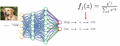
The purpose of the Fully Connected layer is to use these features for classifying the input image into various classes (Dog,Cat) etc based on the training dataset. Here on flatten results, a full ANN (Artificial Neural Network) is applied to get the output values.

Apart from classification, adding a fully-connected layer is also a (usually) cheap way of learning non-linear combinations of these features. Most of the features from convolutional, pooling and flattening layers may be good for the classification task, but combinations of those features might be even better.

The sum of output probabilities from the Fully Connected Layer is always 1. This is ensured by using the Softmax as the activation function in the output layer of the Fully Connected Layer.

The Softmax function takes a vector of arbitrary real-valued output scores (e.g. two y output values shown above) and then squashes them to a vector of values between zero and one that sum to one.

Summary:

• Convolution + Pooling + Flattening layers act as Feature Extractors from the input image while 
• Fully Connected layer acts as a classifier.

C). Softmax & Cross-Entropy:

As mentioned above in Step 4, the sum of output probabilities from the Fully Connected Layer is always 1. This is ensured by using the Softmax as the activation function in the output layer of the Fully Connected Layer.

The Softmax function takes a vector of arbitrary real-valued output scores (e.g. two y output values shown above) and then squashes them to a vector of values between zero and one that sum to one.

Code: Convolutional Neural Network

# Installing Theano/Tensorflow/Kears (As in ANN)
# Part 1 - Building the CNN

# Importing the Keras libraries and packages
from keras.models import Sequential
from keras.layers import Convolution2D
from keras.layers import MaxPooling2D
from keras.layers import Flatten
from keras.layers import Dense

# Initializing the CNN
classifier = Sequential()

# Step 1.1 - Convolution
classifier.add(Convolution2D(32, 3, 3, input_shape = (64, 64, 3), activation = 'relu'))

# Step 1.2 - Pooling
classifier.add(MaxPooling2D(pool_size = (2, 2)))

# Adding a second convolutional layer
classifier.add(Convolution2D(32, 3, 3, activation = 'relu'))
classifier.add(MaxPooling2D(pool_size = (2, 2)))

# Step 1.3 - Flattening
classifier.add(Flatten())

# Step 1.4 - Full connection
# Here we are choosing 'Rectifier' (relu) as an activation function for Hidden Layer
# Here we are choosing 'Sigmoid' as an activation function for Output Layer
classifier.add(Dense(output_dim = 128, activation = 'relu'))
classifier.add(Dense(output_dim = 1, activation = 'sigmoid'))

# Compiling the CNN
# Here optimizer is 'Stochastic Gradient Descent'. One of the SGD Algoritm is 'adam'
# Here loss is 'binary_crossentropy' as result is binay (dog/cat). If there are more output loss would be 'category_crossentropy
classifier.compile(optimizer = 'adam', loss = 'binary_crossentropy', metrics = ['accuracy'])

# Part 2 - Fitting the CNN to the images
# Check Documentation here - https://keras.io/preprocessing/image/
from keras.preprocessing.image import ImageDataGenerator

train_datagen = ImageDataGenerator(rescale = 1./255,
                                   shear_range = 0.2,
                                   zoom_range = 0.2,
                                   horizontal_flip = True)

test_datagen = ImageDataGenerator(rescale = 1./255)

training_set = train_datagen.flow_from_directory('dataset/training_set',
                                                 target_size = (64, 64),
                                                 batch_size = 32,
                                                 class_mode = 'binary')

test_set = test_datagen.flow_from_directory('dataset/test_set',
                                            target_size = (64, 64),
                                            batch_size = 32,
                                            class_mode = 'binary')

# Here 'samples_per_epoch' is the number of images we have in out 'Training Set'
# Here 'nb_val_samples' is the number of images we have in out 'Test Set'
classifier.fit_generator(training_set,
                         samples_per_epoch = 8000,
                         nb_epoch = 25,
                         validation_data = test_set,
                         nb_val_samples = 2000)

Hope this helps!!

Regards,

Arun Manglick

Artificial Neural Networks

Basics:
Here we'll first learn below:

1. Neuron
2. Activation Function
3. How Neural N/w Learn
4. Gradient Descent
5. Stochastic Gradient Descent
6. Back Propagation

1). Neuron:

2). Activation Function:

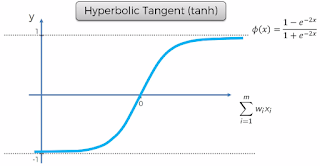
Four Types:
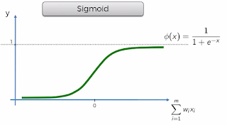
 - Threshold Function (Passes 0 or 1, If X < 0, Then 0, If X >= 0 Then 1)
 - Sigmoid Function (Used in Logistic Regression)
 - Rectifier Function (Mostly Used) (Paper Link)
 - Hyperbolic Tanget (tanh)

In most of the model, Rectifier is applied at 2nd step and Sigmoid is at 3rd step.

3). How Neuron Network Learns:

Steps:

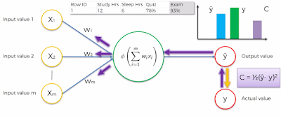
1. Apply Weight to Input Values and Calculate Output Values (y Hat)
2. Determine Cost I.e. variation between actual value (y) and predicted value (y hat)
3. Intent is to minimize cost as much as possible. Thus adjust weight and re-apply and check new cost value
4. Repeat steps until you find zero or minimum cost value

 

The above is applied to one student. If there are multiple student same is applied to all rows in one go and repeated again for all rows in one go, until you find cumulative minimum cost.

4). Gradient Descent:

Gradient descent is a popular method in the field of machine learning and used to find the minimum error by minimizing a "cost" function.

Gradient descent is a first-order iterative optimization algorithm for finding the minimum of a function.

To find a local minimum of a function using gradient descent, one takes steps proportional to the negative of the gradient (or of the approximate gradient) of the function at the current point. If instead one takes steps proportional to the positive of the gradient, one approaches a local maximum of that function; the procedure is then known as gradient ascent.

In easy words to find minimum, move in the way whichever is downhill, take steps and find minimum faster.

5). Stochastic Gradient Descent:

Above is able to find a global minimum where cross function is convex. But what if it's not convex and look like below. In this case, as you see applying above method ends up with incorrect minimum point.

In such case SGD is used.

Stochastic gradient descent (often shortened in SGD), also known as incremental gradient descent, is a stochastic approximation of the gradient descent optimization method for minimizing an objective function that is written as a sum of differentiable functions. In other words, SGD tries to find minima or maxima by iteration.

6). Back Propogation:

Practical:

Here we'll understand below:

• Business Problem
• Installing/Understand
• Theano, 
• Tensorflow and 
• Keras
• Code Implementation

1). Business Problem:
You have bank customers (credit score, country, age, gender, tenure,balance, credit card, loan, exited etc). Given the problem you need to find out which customers are at high risk of leaving the bank.
In summary, it's a Classification Problem.

2). Installation/Understand Theano, TensorFlow, Keras

Theano: At a glance

Theano is an open source numerical computation Python library that allows you to Define, Optimize, and Evaluate mathematical expressions involving multi-dimensional arrays efficiently. Theano can run on CPU or GPU (more useful for neural networks calculations).

Features:

• Tight integration with NumPy - e.g. Theano can use g++ or nvcc to compile parts your expression graph into CPU or GPU instructions, which run much faster than pure Python.
• Transparent use of a GPU – Perform data-intensive computations much faster than on a CPU.
• Efficient symbolic differentiation – Theano can automatically build symbolic graphs for computing gradients.
• Speed and stability optimizations – Get the right answer for log(1+x) even when x is really tiny.
• Dynamic C code generation – Evaluate expressions faster.
• Extensive unit-testing and self-verification – Detect and diagnose many types of errors.

Tensor Flow: 

TensorFlow is an open source software library for numerical computation using data flow graphs. Nodes in the graph represent mathematical operations, while the graph edges represent the multidimensional data arrays (tensors) communicated between them.
The flexible architecture allows you to deploy computation to one or more CPUs or GPUs in a desktop, server, or mobile device with a single API.

TensorFlow computations are expressed as stateful dataflow graphs. The name TensorFlow derives from the operations which such neural networks perform on multidimensional data arrays (tensors).

TensorFlow was originally developed by researchers and engineers working on the Google Brain Team (Nov 2015) for the purposes of conducting machine learning and deep neural networks research.

Used for machine learning across a range of tasks, building and training neural networks to detect and decipher patterns and correlations, analogous to the learning and reasoning which humans use.

In just its first year, TensorFlow has helped researchers, engineers, artists, students, and many others make progress with everything from language translation to early detection of skin cancer and preventing blindness in diabetics.

Keras: 

Keras was developed with a focus on enabling fast experimentation.
Keras library is used to build deep neural network model with very few lines of code.

Keras is a high-level neural networks API, written in Python and capable of running on top of TensorFlow, Theano,  MXNet, Deeplearning4j or CNTK.

Google's (In 2017) TensorFlow team decided to support Keras in TensorFlow's core library. It was explained that Keras was conceived to be an interface rather than an end-to-end machine-learning framework. It presents a higher-level, more intuitive set of abstractions that make it easy to configure neural networks regardless of the backend scientific computing library.

Microsoft has been working to add a CNTK backend to Keras as well.

The library contains numerous implementations of commonly used neural network building blocks such as layers, objectives, activation functions, optimizers, and a host of tools to make working with image and text data easier.

Code: Artificial Neural Network

# Part 1: Data Pre-Processing
# Importing the libraries
import numpy as np
import matplotlib.pyplot as plt
import pandas as pd

# Importing the dataset
dataset = pd.read_csv('Churn_Modelling.csv')
X = dataset.iloc[:, 3:13].values
y = dataset.iloc[:, 13].values

# Encoding categorical data - 'Geography'& 'Gender'
from sklearn.preprocessing import LabelEncoder, OneHotEncoder
labelencoder_X_1 = LabelEncoder()
X[:, 1] = labelencoder_X_1.fit_transform(X[:, 1])

labelencoder_X_2 = LabelEncoder()
X[:, 2] = labelencoder_X_2.fit_transform(X[:, 2])

onehotencoder = OneHotEncoder(categorical_features = [1])
X = onehotencoder.fit_transform(X).toarray()
X = X[:, 1:]  # To avoid dummy variable trap

# Splitting the dataset into the Training set and Test set
from sklearn.model_selection import train_test_split
X_train, X_test, y_train, y_test = train_test_split(X, y, test_size = 0.2, random_state = 0)

# Feature Scaling
from sklearn.preprocessing import StandardScaler
sc = StandardScaler()
X_train = sc.fit_transform(X_train)
X_test = sc.transform(X_test)

# Part2: Now let's make the ANN!
# Importing the Keras libraries and packages
import keras
from keras.models import Sequential
from keras.layers import Dense

# Initializing the ANN
classifier = Sequential()

# Adding the input layer and the first hidden layer
# Here Output_dim denotes number of hidden layers, which is taken as average of input & outout. I.e (11+1)/2 = 6
# Here we are choosing 'Rectifier' (relu) as an activation function for Hidden Layer
# Here we are choosing 'Sigmoid' as an activation function for Output Layer
classifier.add(Dense(output_dim = 6, init = 'uniform', activation = 'relu', input_dim = 11))

# Adding the second hidden layer
classifier.add(Dense(output_dim = 6, init = 'uniform', activation = 'relu'))

# Adding the output layer
classifier.add(Dense(output_dim = 1, init = 'uniform', activation = 'sigmoid'))

# Compiling the ANN
# Here optimizer is 'Stochastic Gradient Descent'. One of the SGD Algoritm is 'adam'
classifier.compile(optimizer = 'adam', loss = 'binary_crossentropy', metrics = ['accuracy'])
classifier.compile()

# Fitting the ANN to the Training set
classifier.fit(X_train, y_train, batch_size = 10, nb_epoch = 100)

# Part 3 - Making the predictions and evaluating the model
# Predicting the Test set results
y_pred = classifier.predict(X_test)
y_pred = (y_pred > 0.5)  # Predictions Less Than 0.5 will be treated as 'False', else 'True'

# Making the Confusion Matrix
from sklearn.metrics import confusion_matrix
cm = confusion_matrix(y_test, y_pred)

Hope this helps!!

Arun Manglick