Basics:
From m independent variables of given dataset, LDA extracts p <= m new independent variables that separate most of the classes of the dependent variables.
Linear discriminant analysis (LDA) is a generalization of Fisher's linear discriminant, a method used in statistics, pattern recognition and machine learning to find a linear combination of features that characterizes or separates two or more classes of objects or events.
LDA is also closely related to PCA in that they both look for linear combinations of variables which best explain the data.
- LDA explicitly attempts to model the difference between the classes of data.
- PCA on the other hand does not take into account any difference in class

Business Problem:
(Same as in PCA) Given 13 independent variables (various type of alcohol) in wine, decide which customer segment will prefer a particular type of wine. Now as it's tough to determine customer segment on bases of so many independent variables, we'll apply PCA and deduce best two independent variables to solve this problem.
Code: LDA
# Importing the libraries
import numpy as np
import matplotlib.pyplot as plt
import pandas as pd
# Importing the dataset
dataset = pd.read_csv('Wine.csv')
X = dataset.iloc[:, 0:13].values
y = dataset.iloc[:, 13].values
# Splitting the dataset into the Training set and Test set
from sklearn.model_selection import train_test_split
X_train, X_test, y_train, y_test = train_test_split(X, y, test_size = 0.2, random_state = 0)
# Feature Scaling
from sklearn.preprocessing import StandardScaler
sc = StandardScaler()
X_train = sc.fit_transform(X_train)
X_test = sc.transform(X_test)
# Applying LDA
from sklearn.discriminant_analysis import LinearDiscriminantAnalysis as LDA
lda = LDA(n_components = 2)
X_train = lda.fit_transform(X_train, y_train) # This is additional here in comparison to LCA
X_test = lda.transform(X_test)
# Fitting Logistic Regression to the Training set
from sklearn.linear_model import LogisticRegression
classifier = LogisticRegression(random_state = 0)
classifier.fit(X_train, y_train)
# Predicting the Test set results
y_pred = classifier.predict(X_test)
# Making the Confusion Matrix
# Used to evauate performance of model to see corret/incorrection predictions made by Logistic regression
from sklearn.metrics import confusion_matrix
cm = confusion_matrix(y_test, y_pred)
# Visualising the Training set results
from matplotlib.colors import ListedColormap
X_set, y_set = X_train, y_train
X1, X2 = np.meshgrid(np.arange(start = X_set[:, 0].min() - 1, stop = X_set[:, 0].max() + 1, step = 0.01),
np.arange(start = X_set[:, 1].min() - 1, stop = X_set[:, 1].max() + 1, step = 0.01))
plt.contourf(X1, X2, classifier.predict(np.array([X1.ravel(), X2.ravel()]).T).reshape(X1.shape),
alpha = 0.75, cmap = ListedColormap(('red', 'green', 'blue')))
plt.xlim(X1.min(), X1.max())
plt.ylim(X2.min(), X2.max())
for i, j in enumerate(np.unique(y_set)):
plt.scatter(X_set[y_set == j, 0], X_set[y_set == j, 1],
c = ListedColormap(('red', 'green', 'blue'))(i), label = j)
plt.title('Logistic Regression (Training set)')
plt.xlabel('LD1')
plt.ylabel('LD2')
plt.legend()
plt.show()

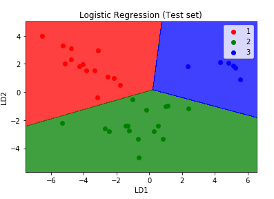
# Visualising the Test set results
from matplotlib.colors import ListedColormap
X_set, y_set = X_test, y_test
X1, X2 = np.meshgrid(np.arange(start = X_set[:, 0].min() - 1, stop = X_set[:, 0].max() + 1, step = 0.01),
np.arange(start = X_set[:, 1].min() - 1, stop = X_set[:, 1].max() + 1, step = 0.01))
plt.contourf(X1, X2, classifier.predict(np.array([X1.ravel(), X2.ravel()]).T).reshape(X1.shape),
alpha = 0.75, cmap = ListedColormap(('red', 'green', 'blue')))
plt.xlim(X1.min(), X1.max())
plt.ylim(X2.min(), X2.max())
for i, j in enumerate(np.unique(y_set)):
plt.scatter(X_set[y_set == j, 0], X_set[y_set == j, 1],
c = ListedColormap(('red', 'green', 'blue'))(i), label = j)
plt.title('Logistic Regression (Test set)')
plt.xlabel('LD1')
plt.ylabel('LD2')
plt.legend()
plt.show()

Hope this helps!!
(Same as in PCA) Given 13 independent variables (various type of alcohol) in wine, decide which customer segment will prefer a particular type of wine. Now as it's tough to determine customer segment on bases of so many independent variables, we'll apply PCA and deduce best two independent variables to solve this problem.
Code: LDA
# Importing the libraries
import numpy as np
import matplotlib.pyplot as plt
import pandas as pd
# Importing the dataset
dataset = pd.read_csv('Wine.csv')
X = dataset.iloc[:, 0:13].values
y = dataset.iloc[:, 13].values
# Splitting the dataset into the Training set and Test set
from sklearn.model_selection import train_test_split
X_train, X_test, y_train, y_test = train_test_split(X, y, test_size = 0.2, random_state = 0)
# Feature Scaling
from sklearn.preprocessing import StandardScaler
sc = StandardScaler()
X_train = sc.fit_transform(X_train)
X_test = sc.transform(X_test)
# Applying LDA
from sklearn.discriminant_analysis import LinearDiscriminantAnalysis as LDA
lda = LDA(n_components = 2)
X_train = lda.fit_transform(X_train, y_train) # This is additional here in comparison to LCA
X_test = lda.transform(X_test)
# Fitting Logistic Regression to the Training set
from sklearn.linear_model import LogisticRegression
classifier = LogisticRegression(random_state = 0)
classifier.fit(X_train, y_train)
# Predicting the Test set results
y_pred = classifier.predict(X_test)
# Making the Confusion Matrix
# Used to evauate performance of model to see corret/incorrection predictions made by Logistic regression
from sklearn.metrics import confusion_matrix
cm = confusion_matrix(y_test, y_pred)
# Visualising the Training set results
from matplotlib.colors import ListedColormap
X_set, y_set = X_train, y_train
X1, X2 = np.meshgrid(np.arange(start = X_set[:, 0].min() - 1, stop = X_set[:, 0].max() + 1, step = 0.01),
np.arange(start = X_set[:, 1].min() - 1, stop = X_set[:, 1].max() + 1, step = 0.01))
plt.contourf(X1, X2, classifier.predict(np.array([X1.ravel(), X2.ravel()]).T).reshape(X1.shape),
alpha = 0.75, cmap = ListedColormap(('red', 'green', 'blue')))
plt.xlim(X1.min(), X1.max())
plt.ylim(X2.min(), X2.max())
for i, j in enumerate(np.unique(y_set)):
plt.scatter(X_set[y_set == j, 0], X_set[y_set == j, 1],
c = ListedColormap(('red', 'green', 'blue'))(i), label = j)
plt.title('Logistic Regression (Training set)')
plt.xlabel('LD1')
plt.ylabel('LD2')
plt.legend()
plt.show()

# Visualising the Test set results
from matplotlib.colors import ListedColormap
X_set, y_set = X_test, y_test
X1, X2 = np.meshgrid(np.arange(start = X_set[:, 0].min() - 1, stop = X_set[:, 0].max() + 1, step = 0.01),
np.arange(start = X_set[:, 1].min() - 1, stop = X_set[:, 1].max() + 1, step = 0.01))
plt.contourf(X1, X2, classifier.predict(np.array([X1.ravel(), X2.ravel()]).T).reshape(X1.shape),
alpha = 0.75, cmap = ListedColormap(('red', 'green', 'blue')))
plt.xlim(X1.min(), X1.max())
plt.ylim(X2.min(), X2.max())
for i, j in enumerate(np.unique(y_set)):
plt.scatter(X_set[y_set == j, 0], X_set[y_set == j, 1],
c = ListedColormap(('red', 'green', 'blue'))(i), label = j)
plt.title('Logistic Regression (Test set)')
plt.xlabel('LD1')
plt.ylabel('LD2')
plt.legend()
plt.show()
Hope this helps!!
Arun Manglick
No comments:
Post a Comment