K-Means Clustering

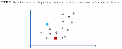
Basics:

K-means clustering aims to partition n observations into k clusters in which each observation belongs to the cluster with the nearest mean, serving as a prototype of the cluster. 

Let's apply this process.

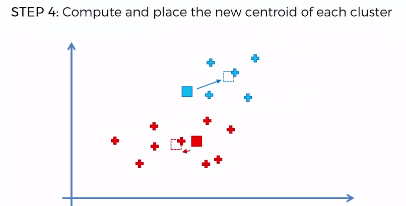
Random Initialization Trap:
Here we'll try to understand how choosing random K Points (Step 2) could result in bad random initialization. Here you'll see for the same problem choosing random K Points, result in two different type of clusters. Solution to this trap is K-Means++

Elbow Method : To Choose Right Number of Clusters:

Given a set of observations (x1, x2, …, xn), where each observation is a d-dimensional real vector, k-means clustering aims to partition the n observations into k (≤ n) sets S = {S1, S2, …, Sk} so as to Minimize the Within-Cluster Sum of Squares (WCSS) (i.e. variance). Formally, the objective is to find minimum WCSS.

Looking at the formula it's evident that if there is one cluster for the below data points, WCSS will be high, in comparison to more than one cluster.

So you see hear more the number of clusters minimum will be WCSS. Just a note if number of clusters are same as number of data points, WCSS will be zero. Thus to choose right number of clusters use the below elbow method where you keep increasing number of clusters and check for WCSS. Wherever you find substantial reduce that will be the optimum number of clusters for your problem.

Code: K-Means Clustering

# For the given problem Age, Salary and Spending score, below code will try to deduce how many customer segments can be created so that business can focus on those segments and create corrective business plans.

# Importing the libraries
import numpy as np
import matplotlib.pyplot as plt
import pandas as pd

# Importing the dataset
dataset = pd.read_csv('Mall_Customers.csv')
X = dataset.iloc[:, [3, 4]].values
# y = dataset.iloc[:, 3].values

# Using the elbow method to find the optimal number of clusters
from sklearn.cluster import KMeans
wcss = []
for i in range(1, 11):
    kmeans = KMeans(n_clusters = i, init = 'k-means++', random_state = 42)
    kmeans.fit(X)
    wcss.append(kmeans.inertia_)

plt.plot(range(1, 11), wcss)
plt.title('The Elbow Method')
plt.xlabel('Number of clusters')
plt.ylabel('WCSS')
plt.show()

# Above plot shows K=5 will be right number of clusters as at K=5 WCSS show substantial decrease
# Fitting K-Means to the dataset
kmeans = KMeans(n_clusters = 5, init = 'k-means++', random_state = 42)
y_kmeans = kmeans.fit_predict(X)

# Visualising the clusters
plt.scatter(X[y_kmeans == 0, 0], X[y_kmeans == 0, 1], s = 100, c = 'red', label = 'Cluster 1')
plt.scatter(X[y_kmeans == 1, 0], X[y_kmeans == 1, 1], s = 100, c = 'blue', label = 'Cluster 2')
plt.scatter(X[y_kmeans == 2, 0], X[y_kmeans == 2, 1], s = 100, c = 'green', label = 'Cluster 3')
plt.scatter(X[y_kmeans == 3, 0], X[y_kmeans == 3, 1], s = 100, c = 'cyan', label = 'Cluster 4')
plt.scatter(X[y_kmeans == 4, 0], X[y_kmeans == 4, 1], s = 100, c = 'magenta', label = 'Cluster 5')
plt.scatter(kmeans.cluster_centers_[:, 0], kmeans.cluster_centers_[:, 1], s = 300, c = 'yellow', label = 'Centroids')
plt.title('Clusters of customers')
plt.xlabel('Annual Income (k$)')
plt.ylabel('Spending Score (1-100)')
plt.legend()
plt.show()

Cluster 1 - Average Income & Average Spending  - Standard Clients
Cluster 2 - More Income & Less Spending - Careful Clients
Cluster 3 - Less Income & Less Spending  - Sensible Clients
Cluster 4 - Less Income & High Spending - Careless Clients
Cluster 5 - High Income & High Spending - Potential Clients

Hope this helps!!

Arun Manglick